1 Braided-channel reorganization during storms, resolved seismically
Glacier-fed mountain rivers carry the floods and sediment that drive downstream hazard, yet they are sparsely gaged and their braided source reaches reorganize during the very floods we most need to observe, a process normally seen only as before/after snapshots. We use near-channel seismic stations along the Puyallup and Nisqually Rivers draining Mt. Rainier, Washington, paired with USGS gages, to monitor the December 2025 Pacific Northwest atmospheric-river (AR) floods. Band-limited seismic power tracks turbulent flow and hence discharge (P\propto Q^{b}, b\approx1–2.5 in the resolvable 1–15 Hz band). The central result is a statistically significant steepening of the P–Q scaling is a fluvial regime transition of geometric channel reorganization, not a bedload onset (reversible hysteresis, no supply decay), and the continuous seismic record resolves its event-scale timing — at matched discharge the source baseline steps up on the falling limb of the main pulse, lagging peak discharge by ~half a day (onset) to a few days, in a stepwise reorganization of the braided Puyallup outwash plain rather than a gradual one. This timing, which gages and satellite snapshots cannot give, is independently corroborated by Sentinel-2/-1 imagery (the active thread migrated toward the most anomalous station). A second basin (Nisqually) shows the same physics is larger but confounded: its gage sits 13–21 km downstream on a far wider, higher braidplain where the post-flood rain→snow supply shutoff masks the geometric signal — together defining the domain in which source-resolved river seismology is clean (a compact channel with a co-located gage). Finally, a deterministic routing of the upstream discharge through the downstream rating reproduces the observed downstream stage for this event and serves as a proof-of-concept for a seismic-fed flood nowcast in this gage-sparse lahar corridor, not yet a skill-validated forecast.
braided rivers, channel reorganization, river discharge, Mt. Rainier, atmospheric river, environmental seismology
2 Introduction
Glacier-fed mountain rivers braid and reorganize their channels during the very floods that matter most for downstream hazard. As discharge rises, braided threads widen, switch, and avulse across the valley floor, redistributing the sediment that aggrades channels, undermines bridges and levees, and charges lahar-prone corridors (Czuba et al., 2012; Hoblitt et al., 1998). Yet we almost never observe this reorganization as it happens: stream gages record discharge at a point downstream of the source, and satellites give only before/after snapshots through cloud, so how and when a braided channel rearranges during a flood — the event-scale dynamics — remains largely unobserved. Passive seismic monitoring of the high-frequency ground motion that rivers radiate offers a continuous, non-contact alternative (Burtin et al., 2008; Cook & Dietze, 2022; Gimbert et al., 2014; Tsai et al., 2012), sensitive to the near-channel processes — turbulent flow and sediment transport — that drive channel change, and recorded at the 10-minute cadence neither gages nor imagery provide for channel position.
Dynamic braiding in pro-glacial rivers.
Geophysical sensing in mountain areas provide an opportunity to observe their dynamics and characterize them with process based approaches.
Two sources dominate the near-channel high-frequency wavefield. Turbulent flow over the bed radiates seismic power that is, to first order, linear in discharge, P_{\text{water}} \;\propto\; Q^{\,b_t}, \qquad b_t \approx 0.9\text{–}1.4 , \tag{2.1}
whereas bedload grain impacts radiate power that is threshold-gated and super-linear in discharge,
P_{\text{bed}} \;\propto\; (Q - Q_c)^{\,b_b}, \qquad b_b > b_t , \tag{2.2}
with Q_c an entrainment threshold. A bedload contribution therefore makes the measured exponent b exceed the turbulence baseline b_t and rise with frequency (Bakker et al., 2020).
Model assumptions behind Equation 2.1–Equation 2.2. These discharge forms are reductions of the physical models, and we list the assumptions they fold in. The turbulence exponent follows from P_{\text{water}}\propto H^{7/3}S^{7/3}\propto u_*^{14/3} (Gimbert et al. 2014) combined with at-a-station hydraulic geometry (H\propto Q^{0.3\text{–}0.6} at fixed slope S), giving b_t\approx1. The bedload form follows from P_{\text{bed}}\propto q_b\,D^{3} with impact flux q_b\propto(\tau_*-\tau_{*c})^{3/2} (Tsai et al. 2012; Bakker et al. (2020)), so b_b inherits the excess-Shields-stress nonlinearity and the strong D^3 weighting toward the coarse grain-size tail. We do not measure flow depth H, shear velocity u_*, Shields stress \tau_*, or grain size D; they enter only as the exponents b_t,b_b and the threshold Q_c, which we estimate empirically. Two further assumptions are implicit and revisited later: that the recorded frequency band actually samples the bedload source (it is set by station Nyquist; §Methods), and that seismic attenuation lets a station sense the channel of interest (§Discussion).
These scalings, and the discharge-proxying, bedload, and hysteresis results built on them, come almost entirely from single-thread channels (Antoniazza et al., 2023; Burtin et al., 2008; Roth et al., 2016; Schmandt et al., 2017), where a fixed line source at a known distance is a fair idealization. A braided glacial reach is the opposite case: the source is a spatially distributed, non-stationary set of active anabranches that migrate and avulse during a flood, breaking the single-channel assumption — but, we argue, also opening a new observable. Because the seismic source moves with the channel, the continuous record carries the timing of the reorganization itself, a quantity that the dense-array braided studies that exist (Burtin et al., 2011; Piantini et al., 2022) localize in space but do not resolve in event time, and that gages and snapshot imagery cannot provide at all.
The December 2025 atmospheric-river floods on Mt. Rainier — near-record discharge on these glacial rivers — provide a natural experiment along a glacial-river transect. We first establish what the network can robustly measure: band-limited seismic power that tracks turbulent flow and therefore discharge. We then pursue the question the continuous, source-proximal record is uniquely able to answer, and which neither gages nor before/after satellite imagery can: (i) when a braided glacial reach reorganizes during a flood, what is the timing of that reorganization relative to the hydrograph — does the active channel switch on the rising limb, at peak, or on recession — and is the steepening of the seismic P–Q scaling at a critical discharge a geometric regime transition rather than the “bedload onset” the field routinely infers? Two further questions frame and bound it: (ii) how does the signal organize in space (source→downstream) and across the successive AR pulses, and can upstream seismic anticipate the downstream flood peak? and (iii) does a bedload contribution emerge at all, given that station bandwidth may not even sample it? As we show, the resolvable band is turbulence-dominated and the canonical bedload band is unsampled, so bedload remains a bounded hypothesis — while the event-scale timing of channel reorganization, the reach geometry that bounds when it is measurable, and the early-warning lead are the robust, novel contributions.
2.1 Flood driver: the December 2025 atmospheric-river floods
The study event was a historic compound atmospheric-river sequence, among the strongest and longest-lasting on record for the Puget Sound region. Two back-to-back ARs made landfall ~8–12 December 2025, delivering on the order of 25 cm of rain in the Cascades (locally more over the multi-week period) and >7 cm in ~10 h at the Paradise station on Mt. Rainier, on top of a warm, rain-on-snow setup. Washington Governor Ferguson declared a statewide emergency (~10 December); tens of thousands were under evacuation orders and hundreds of water rescues were conducted.
The western-draining rivers of Mt. Rainier responded at or near record levels: the Carbon River near Fairfax reached its highest stage in 19 years (a near-record crest), the Puyallup produced historic flooding through Pierce County (Orting, Puyallup), and the Nisqually saw major flooding. Mt. Rainier National Park closed indefinitely after mudslides and road washouts. In our gage record the event built downstream: peak discharge of ≈323 m³/s at Puyallup near Electron (RM 41), ≈371 m³/s on the Carbon, ≈425 m³/s on the Nisqually, and ≈1257 m³/s at Puyallup at Puyallup near the mouth — the latter ~4× the headwater peak (Figure 5.9).
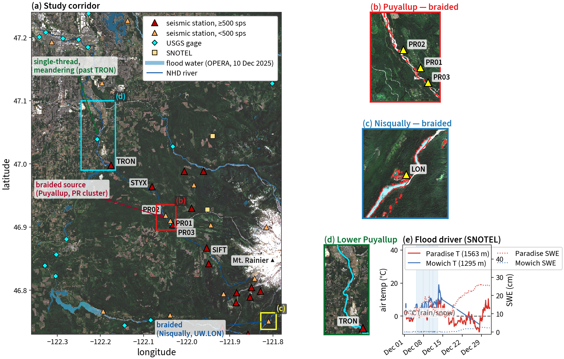
A warm, rain-on-snow driver — and a cold, snow-accumulating aftermath. What made these ARs flood-productive was not rainfall alone but their warmth. At high-elevation SNOTEL stations near the drainage tops — Paradise (1563 m, head of the Nisqually) and Mowich (NW Puyallup/Carbon headwaters) — the AR pulses sat near or above the 0 °C freezing line, so precipitation fell as rain on snow at altitudes that normally store winter snowpack, adding snowmelt to direct runoff (Figure 2.1 e). The contrast with late December is sharp: after ~13 December the high stations dropped well below freezing (Paradise to −9.6 °C) and subsequent storms accumulated as snow — Paradise snow-water-equivalent roughly tripled (≈8→26 cm; Figure 2.1 e) — so comparable precipitation produced little runoff and no comparable discharge or seismic response. The flood-generating window is therefore thermally defined: it is the warm-AR interval, which sets the period over which the seismic–discharge coupling below is evaluated.
This combination — a named, well-documented, near-record AR flood over a glacier-fed volcanic edifice draining toward a densely populated, lahar-hazard lowland (Orting–Puyallup–Tacoma) — makes the event a rare natural experiment for testing seismic flood and sediment monitoring, and is the motivation for the network analysis that follows.
3 Data
The western flanks of Mt Rainier have recently received attention from the hazard community for its recognized threat for massive debris flows and volcanic related lahars (REF). Two seismig monitoring network operates and monitor the volcano-tectonic activities at Mt Rainer: the Cascade Volcano Observatory (network code CC) and the Pacific Northwest Seismic Network (network code UW) stations that are laid out across the western-draining basins of Mt. Rainier — Puyallup, Carbon, Mowich, Nisqually, and upper White. We complement this geophysical monitoring with USGS discharge gages and NRCS SNOTEL/precipitation stations (Figure 2.1). This is a dense (~30-station), multi-basin, multi-sensor network, not a single transect.
The Puyallup River system drains the west flank of Mt. Rainier (Puyallup, Tahoma, and Carbon Glaciers) roughly 54 km to Commencement Bay, Puget Sound. Its lowland floodway is an active sediment sink — repeat aerial-lidar differencing records $1.010^6$ m³ of sand-and-gravel deposition over 2004–2020 ($$60{,}000 m³ yr⁻¹), fed by net erosion of the glacially-charged upper reaches (Anderson, 2026) — an active, supply-rich sediment system routing sediment from eroding source reaches to a depositional lowland. The channel pattern changes systematically downstream (Figure 2.1): the glacial source reaches are multi-thread, braided gravel braidplains — compact at the Puyallup PR cluster (active width tens of m) and far wider on the Nisqually at UW.LON (hundreds of m) — that give way past CC.TRON to a single-thread, meandering channel on the lowland floodplain. This braided-to-single-thread transition frames the source-model problem developed in §sec-braided.
The CC stations are being upgraded from 50 sps to 500 sps high-rate (CH) channels: 19 of 31 stations in the study area now list CH channels (Nyquist 250 Hz) in their metadata (Figure 2.1, marker color). However, these high-rate channels came online in 2026: for the December 2025 event only the legacy 50-sps (BH) waveforms are archived and retrievable (CH returns no data through FDSN at any 2025 date), capping the resolvable band at the 25 Hz Nyquist — below the canonical 30–80 Hz bedload band. The highest-rate near-channel data that do exist for the event are the 100-sps (HH) PNSN/UW broadband stations (UW.RER 0.44 km, UW.LON 0.21 km), which reach a 30–50 Hz lower bedload edge. The 500-sps upgrade is thus a 2026 capability: the same event today would be recorded into the full bedload band — the basis for the “what-if 2026” scenario (§Discussion) — and it also flags that instrument upgrades must be matched by high-rate data archival to realize bedload monitoring. The event peaked at ≈323 m³/s at Puyallup-near-Electron on 2025-12-09.
The satellite images …
The snotel and gage stations.
4 Methods
We process each analysis thread so it can be reproduced from the text below; parameters are pinned in config/analysis.yaml, and the implementing modules are named per thread. Peripheral threads (anthropogenic screening, virtual-discharge inversion, the 30–50 Hz bedload edge, and the coarse/wood-rich caveat) are described in full in the Supplement Texts and pointed to here.
Seismic band-power proxy. Seismic waveforms (IRIS/EarthScope FDSN) are processed in whole-UTC-day blocks. We remove the instrument response to ground velocity (strictly: a day with missing or failed response metadata is dropped rather than silently integrated as raw counts), combine the Z/N/E components as a root-sum-square, and integrate the Welch power spectral density over each frequency band in 10-minute windows to form a band-power proxy P(t). Earthquakes (USGS catalog, M\ge 3.5 within 500 km) and impulsive transients (STA/LTA detection, clipped within the triggered windows only) are removed. We use the 2–8 Hz (flow) and 5–15 Hz (transport-proxy) bands; the 0.5–2 Hz band is excluded because it is dominated by the oceanic secondary microseism rather than river flow. Implemented in src/riverseis/fast_proxy.py.
Robust P–Q fit and hysteresis. Discharge Q(t) comes from USGS NWIS (instantaneous values, m³/s). We align the seismic and discharge series with a high-pass-detrended, sign-constrained constant-lag cross-correlation, which avoids the spurious large lags that arise when the slow storm trend dominates. For each station and band we fit the power law
\log_{10} P \;=\; a \;+\; b\,\log_{10} Q \tag{4.1}
robustly by both ordinary least squares and Theil–Sen, with a MAD outlier clean and bootstrap 95% confidence intervals on b, and quantify event hysteresis with the Lawler index HI (split the series at peak Q and interpolate the rising- and falling-limb power at q_\text{norm}=0.5; positive = clockwise). Implemented in src/riverseis/analysis.py (fit_scaling, lawler_hysteresis_index).
Matched-discharge baseline c(t) and the event-scale timing of channel reorganization (spine). On the braided source reaches the source position is non-stationary, so we separate channel geometry from flow as the residual of the rating, r(t)=\log_{10}P(t)-(a+b\log_{10}Q). This residual is continuous, but it still mixes the geometry signal we want with within-event hysteresis and rating curvature — both functions of Q alone — so reading timing off r(t) directly would confound geometry with flow. We remove the flow dependence by comparing power only at equal discharge. Define a ladder of reference discharges \{Q_k\} (here 60,70,\dots,160 m³ s⁻¹, the band the compound hydrograph re-crosses repeatedly), and let t_{k,j} be the j-th time the hydrograph crosses level Q_k. The matched-discharge baseline is the residual at those crossings, each level referenced to its first (rising-limb) crossing:
c\!\left(t_{k,j}\right) \;=\; r\!\left(t_{k,j}\right) \;-\; r\!\left(t_{k,1}\right), \qquad Q\!\left(t_{k,j}\right)=Q_k . \tag{4.2}
By construction c is therefore not a continuous time series: it is defined only at the discrete instants the hydrograph passes through a reference level, where a true same-stage comparison exists; between crossings the discharge differs and no matched-discharge value is defined. Each c value is a same-stage “snapshot” whose change from the rising-limb reference is source geometry, not discharge. The sampling density in time is set by how often and how long the hydrograph dwells in the reference band, so a fast pulse yields few snapshots and a slow, sustained recession yields many (this is why the slow recession, where reorganization occurs, is also the best-sampled limb; Figure 5.6 a). We detect the onset of reorganization as the first sustained 2\sigma departure of c from the rising-limb band; fit the dominant step with a logistic c_0+\Delta/(1+e^{-(t-t_{50})/\tau}) — midpoint t_{50} giving the lead/lag relative to peak Q, width 4\tau distinguishing a stepwise from a gradual transition, magnitude \Delta its size — and bound t_{50},\tau,\Delta with a moving bootstrap; an end-state offset that returns to zero flags a reversible (non-persistent) excursion rather than an irreversible reorganization.
Flood-wave-lag correction for far-downstream gages. Where a station’s gage is not co-located, gage Q lags the discharge actually passing the station by the flood-wave travel time, inflating the matched-discharge loops. We estimate a constant P–Q lag per station by cross-correlating the limb-timescale (36-h high-passed) components of \log_{10}P and \log_{10}Q — the high pass removes the multi-day storm trend that otherwise locks the correlation onto spurious large lags — and apply it only where a real travel time exists (gage $$3 km away; a co-located gage returns sub-resolution noise); the celerity = distance/lag (Nisqually $$2 m s⁻¹, a physical flood-wave-speed check). A constant lag cannot fully align a multi-kilometre path whose celerity varies with stage, which intrinsically limits matched-discharge timing at a far-gaged reach. Implemented in src/riverseis/analysis.py (estimate_pq_lag, lag_correct); full derivation in Text S2. Finally, because the post-flood rain→snow transition shuts off runoff and the sediment it carries — lowering P at fixed Q for a supply, not geometric, reason — we flag any negative matched-discharge drift that coincides with this basin-wide post-event decline as supply-confounded.
Two-regime broken-stick fit and transport-onset threshold. Bedload is threshold-gated, so the relation should change slope above a critical discharge. We compare a continuous broken-stick fit to a single power law by AIC/BIC. Because consecutive 10-min samples are strongly autocorrelated (\rho\approx0.9–0.99), we score the comparison with an effective sample size n_\text{eff}=n(1-\rho)/(1+\rho) (lag-1 autocorrelation \rho) rather than the raw n; \Delta\mathrm{BIC}>10 is declared significant. We report the breakpoint Q_c and the two exponents b_{<Q_c}\!\to\!b_{>Q_c}.
Attenuation kernel. Power decays as \sim r^{-1}\exp(-2\pi f r/(v_cQ)) with e-folding seismic reach r_e=v_cQ/(2\pi f). Rather than the fluvial default Q\approx20 (Tsai et al. 2012) we adopt a PNW/Rainier-edifice quality factor Q(f)=Q_0 f^{\eta} (Q_0\approx25, \eta\approx0.5 → Q\approx74 at the band center 8.66 Hz; v_c\approx578 m s⁻¹), giving r_e\approx781 m here (vs ~212 m for Q=20).
Satellite channel change and attenuation-weighted illumination. We difference cloud-masked MNDWI =(\text{green}-\text{SWIR})/(\text{green}+\text{SWIR}) wetted-channel maps (water >0) between the pre-flood (Nov 2025) and post-flood (early Jan 2026) epochs, taking the Sentinel-2 optical \cup Sentinel-1 SAR union of active channel, within a 500 m corridor of the NHD mainstem and in UTM 10N. We then propagate the resulting geometry through the manuscript’s own attenuation kernel, summing an attenuation-weighted “wetted illumination” W=\sum_i A_i\,r_i^{-1}\exp(-r_i/r_e) over the active-channel pixels at each station, and read the predicted baseline shift as \Delta\log_{10}P=\log_{10}(W_\text{post}/W_\text{pre}). The water threshold is swept ±0.1 as an ensemble (Text S3). Sentinel-2 true-color basemaps for the figures are cached by workflows/28_fetch_basemaps.py.
Width–stage. The SAR wetted-width proxy per epoch is compared against the continuous gage stage; the secant dW/dH is computed separately on the rising and falling limbs.
Frequency sampling — an important caveat. Turbulent flow dominates the seismic wavefield at ~1–20 Hz and bedload impacts at higher frequencies, with the bedload band conventionally placed at 30–80 Hz (Tsai et al. 2012; Bakker et al. (2020)). Our upper-transect broadband stations (network CC) sample at 50 sps (Nyquist 25 Hz), so they cannot reach the canonical bedload band: our 5–15 Hz “bedload” proxy in fact sits in the turbulence-to-bedload transition and is partly turbulence-controlled. Accessing the true 30–80 Hz band requires ≥160-sps instruments; the only such stations on the corridor are the lowland urban accelerometers (100–200 sps), several of which are traffic-polluted. We therefore interpret the upper-station exponents as a transition-band bedload indicator and separately analyze the high-rate lowland stations in the 30–80 Hz band (§Results) to probe genuine bedload frequencies, accepting their anthropogenic-noise penalty.
Peripheral methods (Supplement Texts). Candidate lowland stations are screened for anthropogenic contamination by the weekday/daytime-vs-night cycle of 4–12 Hz power, restricting the usable transect to the river-dominated broadband network (Text S1; workflows/04_traffic_noise.py). Each river-proximal station is inverted to a seismic virtual discharge Q_\text{seis}=10^{(\log_{10}P-a)/b} and scored against the co-located gage by Nash–Sutcliffe efficiency (Text S4). The 30–50 Hz lower bedload edge from the 100-sps UW broadband stations and the Hertzian contact-frequency argument are in Text S5; the coarse/wood-rich band-lowering caveat is in Text S6.
5 Results
workflows/02_make_figures.py.
| station | band | b | b_lo | b_hi | r | n | HI |
|---|---|---|---|---|---|---|---|
| CC.CARB | 2-8 | -0.31 | -0.33 | -0.30 | -0.38 | 8883 | 0.01 |
| CC.CARB | 5-15 | -0.24 | -0.25 | -0.23 | -0.35 | 8830 | 0.02 |
| CC.GTWY | 2-8 | 1.44 | 1.41 | 1.46 | 0.89 | 8916 | 0.03 |
| CC.GTWY | 5-15 | 1.42 | 1.39 | 1.44 | 0.76 | 8916 | 0.04 |
| CC.PR01 | 0.5-2 | -0.40 | -0.42 | -0.39 | -0.47 | 8916 | -0.01 |
| CC.PR01 | 5-15 | 0.79 | 0.77 | 0.81 | 0.69 | 8340 | -0.03 |
| CC.PR02 | 0.5-2 | 0.12 | 0.09 | 0.14 | 0.12 | 5548 | -0.05 |
| CC.PR02 | 5-15 | 1.80 | 1.78 | 1.81 | 0.96 | 5574 | -0.06 |
| CC.PR03 | 2-8 | 1.59 | 1.58 | 1.60 | 0.98 | 8824 | -0.05 |
| CC.PR03 | 5-15 | 1.71 | 1.70 | 1.72 | 0.98 | 8824 | -0.05 |
| CC.SIFT | 0.5-2 | -0.10 | -0.13 | -0.07 | -0.06 | 8916 | -0.02 |
| CC.SIFT | 5-15 | 0.77 | 0.71 | 0.81 | 0.32 | 8916 | 0.02 |
| CC.STYX | 0.5-2 | 0.65 | 0.63 | 0.67 | 0.63 | 4300 | -0.02 |
| CC.STYX | 2-8 | 1.32 | 1.31 | 1.33 | 0.94 | 8738 | -0.05 |
| CC.STYX | 5-15 | 1.51 | 1.49 | 1.52 | 0.90 | 8738 | -0.05 |
| CC.TRON | 0.5-2 | -0.94 | -0.97 | -0.91 | -0.55 | 4284 | -0.03 |
| CC.TRON | 2-8 | 0.07 | 0.04 | 0.10 | 0.06 | 8798 | -0.01 |
| CC.TRON | 5-15 | 0.56 | 0.54 | 0.58 | 0.52 | 8793 | 0.00 |
| UW.LON | 2-8 | 1.71 | 1.68 | 1.74 | 0.88 | 5472 | -0.00 |
| UW.LON | 5-15 | 1.98 | 1.95 | 2.02 | 0.85 | 5472 | -0.01 |
| UW.RER | 1-5 | 0.03 | 0.01 | 0.05 | 0.03 | 4297 | -0.01 |
| UW.RER | 10-30 | 0.84 | 0.81 | 0.88 | 0.46 | 4297 | -0.09 |
| UW.STOR | 10-30 | 0.14 | 0.12 | 0.16 | 0.21 | 3314 | 0.04 |
| UW.STOR | 2-8 | 0.14 | 0.11 | 0.17 | 0.18 | 3314 | 0.04 |
| UW.UPS | 10-30 | 0.01 | -0.02 | 0.03 | 0.01 | 4136 | 0.02 |
| UW.UPS | 2-8 | 0.01 | -0.02 | 0.03 | 0.01 | 4136 | 0.02 |
5.1 Seismic power tracks discharge
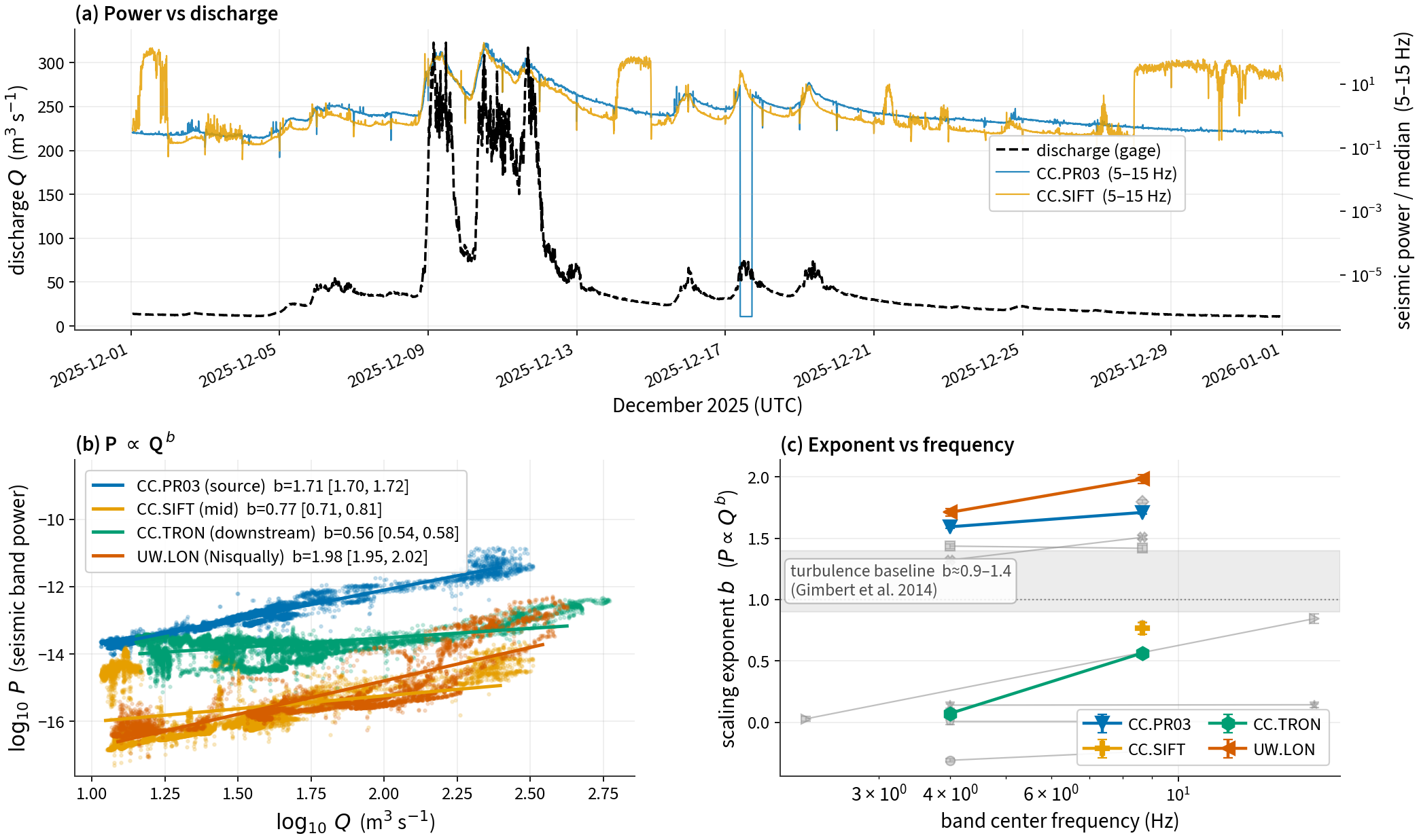
The robust backbone of the analysis is a transect of turbulent-flow seismic power that tracks discharge through the compound AR flood. Seismic band power follows the hydrograph at every clean station — faint in the low-frequency flow band, solid in the high-frequency transport band — with a clear AR2 maximum and downstream decay (Figure 5.1 a).
Frequency-dependent steepening. At the glacial-source station CC.PR03 the exponent rises from b=1.59 (2–8 Hz, r=0.98) to b=1.71 (5–15 Hz, r=0.98), above the turbulent-flow baseline (Figure 5.1 b,c) — a candidate bedload contribution superimposed on turbulence (bounded as a frequency-limited hypothesis in §sec-bedload).
Spatial decay. In the 5–15 Hz bedload band the exponent decays from the glacial source downstream and away from the channel: b=1.71–1.80 at the near-channel Electron stations (CC.PR03, CC.PR02), b=0.79 at CC.PR01 (0.7 km off-channel), b=0.77 (r=0.32) at the off-mainstem tributary station CC.SIFT (~7.5 km off the mainstem), and b=0.56 (r=0.52) at CC.TRON ~20 km downstream and 5.2 km from the channel. The high-frequency excess over the turbulence baseline is therefore confined to the near-source reach and falls to (or below) baseline downstream — an internal contrast indicating the response is source-specific rather than a generic flow artifact.
Where river seismology works — and where it does not. Across all 13 analyzed stations (best flow band, December 2025), 6 yield a usable river signal (r\ge0.7): the Puyallup source cluster (CC.PR01/PR02/PR03, CC.STYX) and both Nisqually stations (CC.GTWY r=0.77, UW.LON r=0.91) — so the method generalizes to a second basin. Two are marginal (CC.SIFT, CC.TRON; r\approx0.6), and three show no signal: CC.CARB (Carbon, 1.7 km off-channel, r\approx-0.2), UW.RER (high on the edifice, far from its gage), and the urban UW.UPS. We plot the no-signal stations alongside the rest (hollow/grey) rather than hide them, and mark them on the map (Figure 2.1, hollow triangles) to document where river seismology was attempted and did not work — itself a useful deployment guide. Notably, the steepest scaling is on the Nisqually (UW.LON b\approx1.98), exceeding the Puyallup source (b\approx1.71).
5.2 Transport-onset threshold and rating geometry
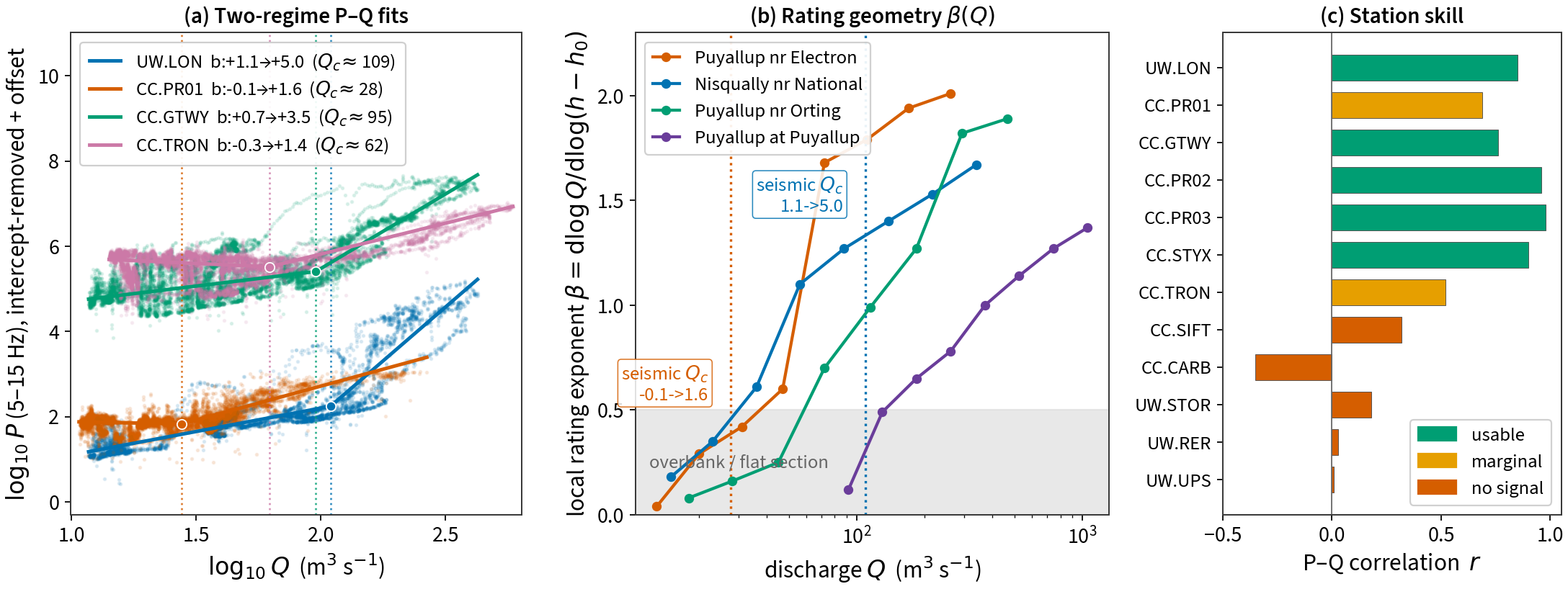
Bedload is threshold-gated, so the seismic-power–discharge relation should change slope above a critical discharge. We compare a continuous broken-stick fit (Figure 5.2 a) to a single power law by AIC/BIC. Because consecutive 10-min samples are strongly autocorrelated (\rho\approx0.9–0.99), we score the comparison with an effective sample size n_\text{eff}=n(1-\rho)/(1+\rho) ($$50–310) rather than the raw n, so a two-segment fit is not declared significant by sheer sample count. Computed over the entire month (flood plus the post-flood low-runoff period, so all stations are treated identically), seven stations cross \Delta\mathrm{BIC}>10, but two — CC.CARB and CC.SIFT — are poorly correlated with discharge (|r|<0.4) and return degenerate fits, leaving five robust river-signal breaks, which we report as two exponents (b_{<Q_c}\!\to\!b_{>Q_c}; starred in Figure 5.1). Four steepen — CC.PR01 (Q_c\approx28 m³/s, b\!:\!-0.12\!\to\!1.59, \Delta\mathrm{BIC}\approx154), CC.TRON (Q_c\approx62, -0.27\!\to\!1.45), and both Nisqually stations CC.GTWY (Q_c\approx95, 0.71\!\to\!3.50) and UW.LON (Q_c\approx109, 1.10\!\to\!5.05 — the steepest above-threshold slope in the network) — while CC.STYX flattens (Q_c\approx27, 2.10\!\to\!1.25). The clean source anchors CC.PR03 and CC.PR02 show no significant break: a single power law suffices. The steeper onsets on the Nisqually match the slope-dependent critical Shields stress (\tau^*_c=0.15\,S^{0.25}; Lamb et al. 2008), which predicts higher thresholds on steeper, coarser reaches.
Candidate mechanisms. A steepening break — power becoming far more sensitive to discharge above Q_c — admits several non-exclusive fluvial mechanisms: (i) bedload entrainment above the critical Shields stress, the classic super-linear excess-stress transport onset (Tsai et al. 2012); (ii) a geometric wetted-front / anabranch activation, where a broad, close, or newly-wetted channel switches on at high stage and adds power without the bed mobilizing — the braided-reach reading we develop for CC.PR01 below (§sec-braided), and a leading candidate for the very steep Nisqually breaks; and (iii) an overbank/floodplain transition past bankfull. A flattening break (CC.STYX) is the opposite signature: above Q_c the flow widens and shallows (or supply saturates), and because turbulent power scales as H^{7/3}, spreading a given discharge across a wider, shallower section suppresses the exponent. Because the resolvable band is turbulence-dominated, every breakpoint is a candidate onset — geometric or bed-mechanical — separated by the satellite channel-change test, which finds the two satellite-tested breaks (CC.PR01 and the steep Nisqually UW.LON) to be substantially geometric, with the larger channel migration falling at the steeper break (an ordering across the two tested reaches, not a fitted relationship; §sec-braided, Figure 5.4), and to be retested out-of-sample on the March-2026 event.
Independent evidence from the gage ratings. The USGS stage–discharge ratings record the same geometry change hydraulically, independent of the seismic data. The local rating exponent \beta(Q)=\mathrm{d}\log Q/\mathrm{d}\log(h-h_0) (from Q=C(h-h_0)^{\beta}) reads whether the conveying section is confining and deepening (\beta rising) or spreading overbank (\beta flat). At the confined source gages \beta climbs steeply with discharge — from $$0.1 at low flow to $$2.0 (Puyallup nr Electron, 0.04→2.01) and $$1.7 (Nisqually nr National, 0.18→1.67) — and the seismic P–Q break Q_c falls within the rating-steepening band at each (Electron Q_c\approx28 m³ s⁻¹, on the \beta\!:\!0.4\!\to\!1.7 ramp; Figure 5.2 b). That an independent hydraulic-geometry transition occurs near the seismic break — at a gage co-located with the source cluster — is direct support for reading the break as geometric rather than bed-mechanical. The lowland Puyallup-at-Puyallup gage instead keeps \beta\lesssim1.4 (≈1.37) even at 10^3 m³ s⁻¹, the flat signature of overbank spreading onto the floodplain — the overbank end-member named among the candidate mechanisms above. A four-gage stage–discharge rating that the seismic virtual discharge can be mapped through is given in Figure 2.12.
5.3 The braided source: a distributed, non-stationary signal
The single most consequential geomorphic caveat to everything above is hiding in plain sight: the Puyallup source cluster (CC.PR01/PR02/PR03, within $$1.5 km of one another) sits on a mobile, sediment-charged glacial-outwash braidplain, not the single, fixed channel that the governing models assume. This is not an assumption: two decades of repeat aerial-lidar differencing (2002–2022) document persistent channel reorganization and bank erosion along these upper Puyallup valley reaches, which act as net sediment sources — feeding the documented aggradation of the lowland floodway downstream — as the deglaciating headwaters shed sediment (Anderson, 2025, 2026; Czuba et al., 2012); the braidplain is demonstrably mobile and supply-charged on the timescale between events. Its bed is poorly-sorted, coarse glacial outwash — sand through boulders, delivered by debris flows and meltwater from the deglaciating headwall — so the reach is supply-rich rather than supply-limited: coarse sediment is effectively always available, and a discharge-threshold “transport onset” is not the expected control (we return to this in interpreting the breaks). Both the turbulent-flow model (Gimbert et al., 2014) and the impact model (Tsai et al., 2012) idealize the source as a single line channel at a known, stationary distance r, with power decaying as \sim r^{-1}\exp(-2\pi f r / v_c Q). A braided reach violates this in ways that the fluvial-seismology calibration literature — built almost entirely on single-thread channels — has rarely had to confront. We argue this is a distinct interpretive regime that deserves its own treatment.
Why braiding changes the physics. (i) The source is spatially distributed across multiple simultaneously active anabranches spread over a valley floor that can exceed the e-folding attenuation length (r_e\approx781 m at band center). The station therefore senses an attenuation-weighted sum dominated by whichever thread is momentarily closest, not by the total discharge. (ii) Discharge partitioning among threads is strongly nonlinear in stage: as stage rises, threads widen, coalesce, and the wetted front jumps laterally — a purely geometric way to manufacture a steepening P–Q break that mimics a transport onset. (iii) Splitting a given Q into N wide, shallow threads lowers per-channel depth H, and because turbulent power scales as H^{7/3}, the braided sum is suppressed relative to a confined channel and the exponent flattens. This prediction is consistent with the observed exponents: the braidplain-central CC.PR01 flattens to b\approx0.79 against b\approx1.7–1.8 at the confined near-channel stations (CC.PR02/PR03; Figure 5.1), the direction braided hydraulic geometry expects when flow partitions into wide, shallow threads (P. Ashmore, 2013). We present it as consistent, not diagnostic, because the same off-channel station also sits farther from the active threads, and distance independently lowers b (§sec-backbone) — the two effects are not separable from b alone. (iv) Braided threads avulse and migrate between and during floods, so the dominant source relocates — imposing a non-stationary distance r and resetting the calibration constant. These are the textbook behaviors of braided gravel-bed rivers — bar growth and dissection, chute cutoff, thread switching, and the lowering of per-thread depth as flow partitions (P. Ashmore, 2013; P. E. Ashmore, 1991) — whose mobility the non-cohesive, sparsely vegetated glacial-outwash banks actively permit (vegetation and bank cohesion are what stabilize single-thread channels; Tal & Paola (2007)).
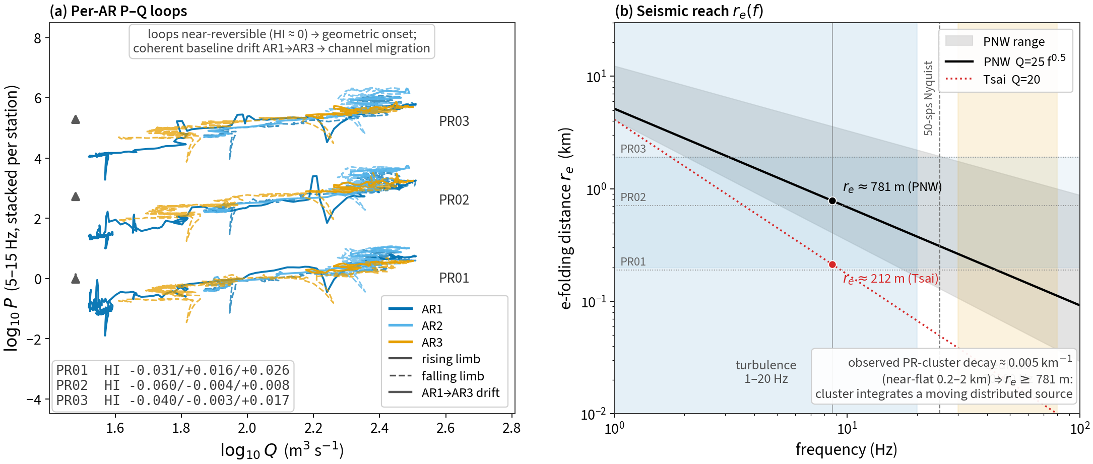
These expectations match the data. Of the three co-located stations, the most braidplain-central, CC.PR01 has the flattest exponent (b=0.79, below the turbulence baseline), the lowest correlation (r=0.69 vs 0.96–0.98), and one of the sharpest broken-stick breaks in the network (b:-0.12\!\to\!1.59 at Q_c\approx28 m³/s, \Delta\mathrm{BIC}\approx154; Figure 5.2). Read naively, that break is the cleanest “bedload onset” we have. But a rising-vs-falling-limb diagnostic (Figure 5.3 a) complicates that reading: the per-AR P–Q loops are reversible (Lawler hysteresis index |HI|\le0.06, no clockwise sense) and the in-window peak power does not decline across successive ARs. Reversibility and the absence of decline rule out a supply-exhaustion (supply-limited) transport onset (cf. the clockwise sediment hysteresis of Burtin et al., 2008; Roth et al., 2016) — but not transport as such: this glacial-outwash braidplain is sediment-rich (the deglaciating headwaters oversupply it; Anderson (2026)), and a supply-unlimited bedload onset would likewise be reversible and non-declining, so hysteresis alone cannot exclude it. The positive case for a geometric wetted-front onset — at Q_c a broad, close, active flow front switches on, not the bed — rests instead on the independent satellite channel-change (§sec-satellite) and on the H^{7/3} flow-partitioning argument above; and in a supply-rich basin a discrete bed-mechanical threshold is the less expected behavior to begin with.
What is present is a coherent baseline drift across the AR sequence: at matched discharge the 5–15 Hz power rises by $0.2–0.3 log units ($2×) from AR1 to the AR2–AR3 plateau at all three stations simultaneously (Figure 5.3 a). A whole-cluster shift at fixed Q is the signature of the active thread migrating toward the stations over the event sequence — i.e. avulsion/lateral reworking of the braidplain, exactly the instability proglacial braided systems are known for (P. Ashmore, 2013; P. E. Ashmore, 1991). This is the first-order risk to the seismic virtual-discharge rating: a calibration learned on December 2025 may not transfer to a later event if the channel has moved, independent of any change in the flow itself.
This connects directly to the only dense-array study of a braided reach to date. Using 80 seismometers across a 600 m braided segment of the Séveraisse (French Alps), Piantini et al. (2022) located impulsive sources to the bend apex of a single active branch — direct evidence that the seismic source in a braided reach lives on specific, migrating anabranches rather than the whole wetted area. The pioneering braided-river seismic study (Burtin et al., 2011, torrent de St Pierre) likewise had to contend with multiple channels in attributing $$3–9 Hz power to turbulent flow. The lesson for a single regional station like ours is sharper than for a dense array: we cannot resolve which anabranch radiates, so we necessarily integrate a non-stationary, attenuation-weighted sum — and must treat braided-reach exponents, thresholds, and ratings as reach-geometry-dependent and event-specific rather than universal grain-mechanical constants.
Seismic reach and weak observed decay. A first-order test on the same-source PR cluster (PR03/PR01/PR02 at 0.19/0.71/1.9 km) finds the 5–15 Hz power nearly distance-independent over 0.2–2 km — an observed decay of $0.005 km⁻¹, far weaker than the PNW prediction (r_e$ m vs the Tsai 212 m; Figure 5.3 b) — implying the band retains less-attenuated lower-frequency (turbulence) energy and that the cluster integrates a moving, distributed source.
5.4 Satellite corroboration of thread migration, two basins
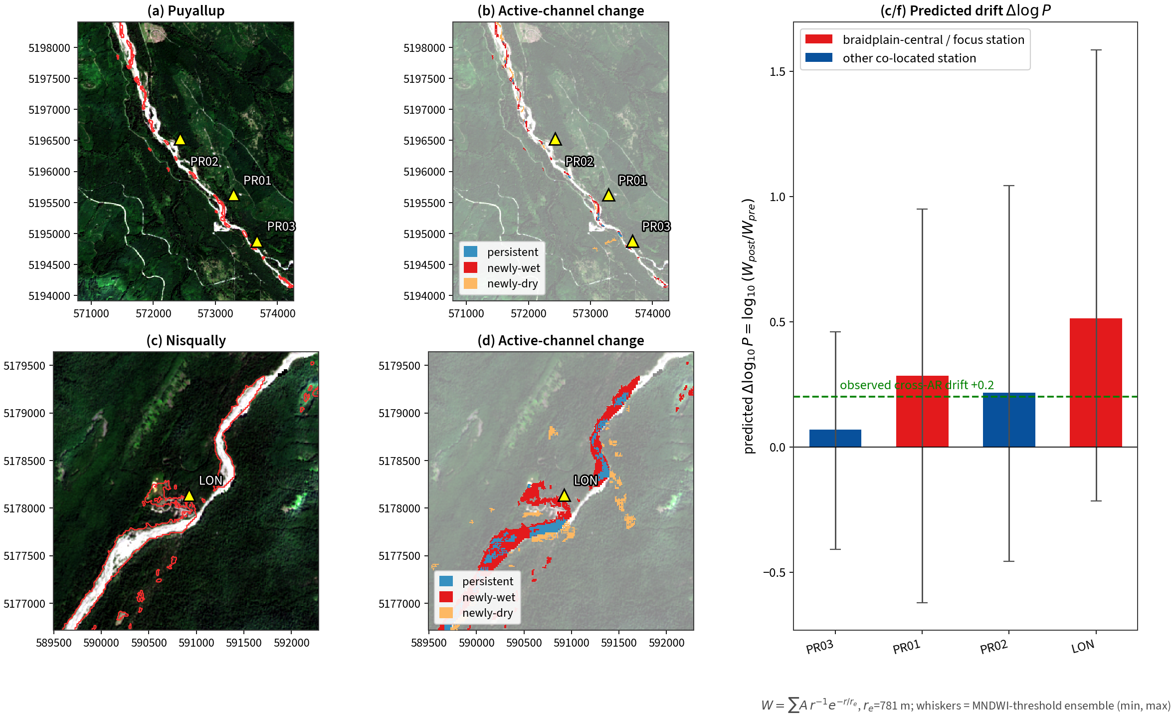
Satellite test of the avulsion prediction. The avulsion reading makes a falsifiable, geometric prediction: if the cross-AR baseline drift is the active thread migrating toward the cluster, then the wetted channel nearest CC.PR01/PR02/PR03 should have moved closer between the pre-flood (November 2025) and post-flood (early January 2026) states, and the implied change should be largest at the most braidplain-central station, CC.PR01. We test this directly with optical and radar imagery (Sentinel-2 L2A and Sentinel-1 RTC, via the Microsoft Planetary Computer), differencing cloud-masked MNDWI wetted-channel maps and VV-backscatter water masks between the two epochs within a 500 m corridor of the NHD mainstem (Figure 5.4 a,b). We then propagate the resulting channel geometry through the manuscript’s own attenuation kernel, summing an attenuation-weighted “wetted illumination” W=\sum_i A_i\,r_i^{-1}\exp(-r_i/r_e) over the active-channel pixels at each station (r_e\approx781 m, §Methods), and read the predicted baseline shift as \Delta\log_{10}P=\log_{10}(W_\text{post}/W_\text{pre}).
The result corroborates the avulsion interpretation in sign and in spatial order, but not yet in absolute magnitude. The active channel reorganized markedly across the event; CC.PR01’s nearest active thread moved $$50 m closer (264→214 m, \Delta r_\text{near}\approx-50 m), and CC.PR01 shows the largest predicted geometric drift of the three stations (median \Delta\log_{10}P\approx+0.28; CC.PR02 +0.22, vs +0.07 at the on-channel anchor CC.PR03), the same rank order and the same positive sign as the observed +0.2-log cross-AR drift (Figure 5.4 c). That the flattest-exponent, lowest-correlation station is also the one the imagery says was most geometrically reworked is independent support that CC.PR01’s anomaly — and the shared baseline drift — is a moving-source effect, not a bed-mechanical one. The magnitude, however, is not robust: because turbid braided water sits near MNDWI$$0, sweeping the water threshold spreads the predicted drift across roughly [-0.6,+1.0] log units (whiskers, Figure 5.4 c), and part of the larger post-flood wetted area is seasonal winter baseflow rather than avulsion. At the 10 m resolution of Sentinel the test therefore confirms the direction and localization of the channel-migration effect while leaving its calibrated magnitude — the conversion of seismic baseline drift into a metric channel-migration distance — for higher-resolution (≈3 m) imagery. The qualitative verdict stands: on a braided reach the seismic virtual-discharge rating is reach-geometry-dependent and can drift between events as the channel moves, exactly the caution §sec-braided raises.
A time-resolved corollary, limited to the cloud-penetrating Sentinel-1 record (optical is cloud-blind through the flood — zero clear Sentinel-2 scenes 1–20 Dec), tracks each off-channel station’s wetted illumination relative to the on-channel anchor CC.PR03 through the AR sequence (Figure 2.10). The braidplain-central CC.PR01 is preferentially illuminated as flow rises, peaking during the AR maximum — the geometric flow-front response in time — although SAR’s under-detection of shallow braided water at 10 m leaves the inter-epoch trend noisy and the net permanent migration better measured by the Nov→Jan bracket above. We treat this as supporting, not primary, evidence.
The geometric mechanism generalizes to a second basin — and scales with the break. The same satellite test, run on the Nisqually reach at UW.LON (Figure 5.4, bottom row), finds a much larger reorganization: the active channel migrated $$240 m toward the station between November and January (robustly inward across all water thresholds; the nearest active thread reaches the station footprint by January, \Delta r_\text{near}\approx-240 m), versus $$50 m at the Puyallup CC.PR01. This matters because UW.LON has the steepest P–Q break in the network (b\!:\!1.1\!\to\!5.0, §sec-threshold) — far steeper than CC.PR01’s (-0.12\!\to\!1.59). The two satellite-tested reaches are, then, consistent with larger channel migration at the steeper break (CC.PR01: \Delta r\approx-50 m, \Delta b\approx+1.7; UW.LON: \Delta r\approx-240 m, \Delta b\approx+4.0) — the direction expected if these breaks are geometric channel-reorganization signatures rather than bed-mechanical transport onsets, with the predicted drift rising across stations (CC.PR03 +0.07, CC.PR02 +0.22, CC.PR01 +0.28, UW.LON +0.52). With only two reaches this is a suggestive ordering, not an established scaling; testing it requires more satellite-instrumented braided breaks. The Nisqually’s large migration partly reflects post-flood (early-January) seasonal wetting and the magnitude is threshold-sensitive, as on the Puyallup; but the inward sense and its order across basins are robust, and they extend the braided-source interpretation — and the caution it implies for virtual-discharge ratings — beyond the Puyallup to a second, independent glacial-river network. The compact, incised Puyallup channel (active width $17–44 m) and the far wider, unconfined Nisqually braidplain ($190–620 m) thus reorganize by the same physics on very different geometric scales, the geomorphic contrast behind the domain law in §sec-domain.
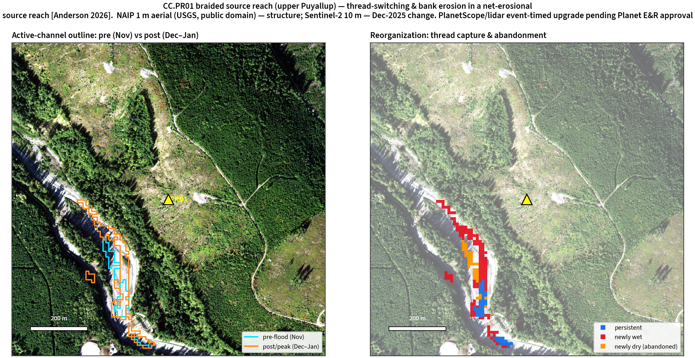
A close-up of the CC.PR01 braidplain makes the reorganization directly legible (Figure 5.5): between the pre-flood image and the post-flood bracket the active channel widens and threads are captured and abandoned around the station. Read through Anderson (2026) — which shows this upper-Puyallup reach to be a net-erosional sediment source (bank erosion, persistent reorganization) that feeds the aggrading lowland downstream — the pattern is one of lateral thread-switching and bank erosion, not local vertical accretion. The basemap is 1-m NAIP aerial imagery (USGS, public domain), which resolves the braided gravel threads and vegetated banks; the December-2025 pre→post active-channel change is bracketed by 10-m Sentinel-2. An event-timed high-resolution version — $$3-m PlanetScope, or a repeat-lidar DEM-of-Difference (Anderson, 2025) — would resolve the reorganized threads at the flood itself and is the planned upgrade.
5.5 Event-scale timing of reorganization and the recession-deposition mechanism
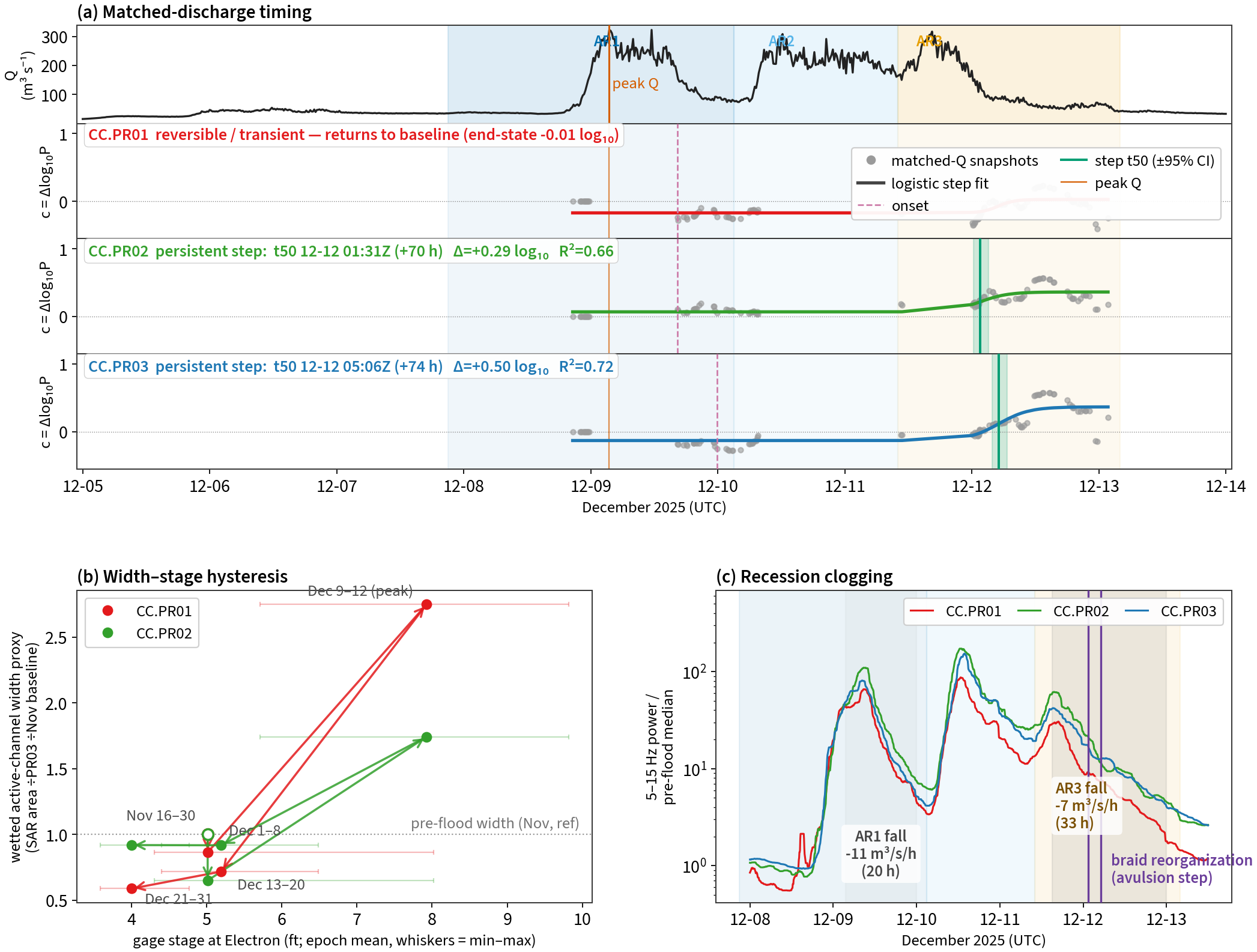
The cross-AR baseline drift establishes that the braid reorganizes; the continuous, sub-daily seismic record additionally resolves when — a question neither gages nor before/after satellite snapshots can address. We isolate the geometry signal as the part of seismic power not explained by discharge, the residual r(t)=\log_{10}P-(a+b\log_{10}Q) about the pooled P–Q rating, and track it at matched discharge: sampling r each time the compound hydrograph crosses a set of reference levels and referencing each level to its first (rising-limb) crossing, so the surviving change is source geometry, not flow (Figure 5.6 a). At the co-located Puyallup cluster the matched-discharge baseline is flat through the rising limb and peak and then steps up on the falling limb of the main pulse — onset $$13–20 h after peak discharge — with the dominant, persistent shift completing on the final recession a few days later (dominant step t_{50}\approx+70 h, CC.PR02 \Delta+0.29, R^2 0.66; \approx+74 h, CC.PR03 \Delta+0.50, R^2 0.72). The transition is stepwise (narrower than a day) rather than a gradual ramp, and it is persistent at the two near-channel stations (CC.PR02/PR03, +0.2–0.3 log) while CC.PR01 — the most braidplain-central — shows a large but reversible excursion, consistent with a thread that shifted and partly re-occupied. We use two terms deliberately: avulsion for the abrupt (sub-daily) thread switch that the seismic step resolves on the event timescale, and migration/relocation for the net Nov→Jan displacement of the dominant thread that the satellite bracket measures — which may itself be a single avulsion or cumulative lateral reworking, a distinction the present data cannot fully settle. The step’s sub-daily width is what identifies it as the abrupt class. Reorganization here is therefore a recession-phase phenomenon, not a rising-limb or at-peak one; its mechanism — recession deposition clogging the active thread and forcing the switch — is developed below, and we keep it separate from the timing result here. We are not aware of a prior seismic study that resolves the event-scale timing of braided-channel reorganization in the field — flume experiments image braided sediment dynamics seismically (Piantini et al., 2022) and field studies bracket channel change with before/after surveys, but neither resolves when within an event — though we state this as “to our knowledge,” not a settled priority claim. The estimate carries honest limits: with three stations and a compound hydrograph that samples matched discharge densely only at the AR limbs, the inter-pulse trough, and the final recession, the precise mid-transition time is pulled toward the largest (final-recession) increment, so the onset (\sim+13 h) is the more robust “when it starts” and the dominant step (\sim+70 h) the “when it is mostly done.”
The falling limb carries information a threshold cannot. A binary entrainment threshold Q_c is, at these source stations, exceeded throughout the multi-day flood recession (Q_c\approx13–28 m³ s⁻¹, far below the recession discharges; Figure 5.2): it labels the entire falling limb “transport-on” and says nothing about how the bed evolves as stage drops. The continuous seismic record does carry that evolution, and — as the rapid AR1 versus sustained AR3 recessions show (Figure 5.6 c) — it is the shape of the recession, not a threshold crossing, that distinguishes a falling limb which merely drains from one slow enough to deposit and reorganize. (Consistent with this being a geometric/transport rather than a strong supply-exhaustion signal, the per-AR loops are near-reversible, |HI|\le0.06.)
A recession-deposition mechanism for the timing. Why does the reorganization fall on the recession rather than the rise? A geomorphic mechanism is available and is testable from the hydrograph shape. On this supply-rich glacial-outwash braidplain — where coarse sediment is effectively unlimited, so a discharge-threshold “transport onset” is not the expected behavior — the relevant event is deposition, not entrainment: as a falling limb drops the bed shear stress below the competence for the coarse load, gravel drops out in the active thread, aggrades and superelevates it, and the flow eventually avulses to a lower, steeper path. This is the classic aggradation/superelevation route to avulsion (Jerolmack & Mohrig, 2007; Mohrig et al., 2000; Slingerland & Smith, 2004), here driven by recession rather than long-term aggradation — a local, thread-scale deposition fully compatible with this upper reach being a net-erosional sediment source at the decadal scale (§sec-braided; Anderson (2026)). The mechanism predicts that reorganization should concentrate on slow, sustained recessions (long residence at moderate stage → more deposition) rather than rapid ones — and that is what the data show (Figure 5.6 c): the Dec-9 (AR1) falling limb is fast (−11.4 m³ s⁻¹ h⁻¹, 20 h; 323→88 m³ s⁻¹) and hosts no persistent step, whereas the sustained Dec-11→13 (AR3) recession is ~40% slower (−6.6 m³ s⁻¹ h⁻¹, 33 h) and is exactly where the persistent reorganization step lands (CC.PR02 12-12 01:31, CC.PR03 12-12 05:06). The satellite change map is consistent — and quantitative: within 300 m of CC.PR01 there are no persistent-water pixels between November and January (0 persistent, 71 newly-wet, 20 newly-dry; Figure 5.4 b, Figure 5.5) — the wetted active thread relocated completely, its abandoned pre-flood course the newly-dry signature the deposition-driven avulsion predicts. We present this as the parsimonious mechanism, not a unique one: the stepwise seismic signature is equally compatible with the other geometric routes to braid change — discrete thread abandonment, bar dissection, or chute cutoff (P. E. Ashmore, 1991) — and rests on a single compound event. Whether the recession-phase timing holds for the more frequent, moderate floods that do most of the cumulative geomorphic work (Wolman & Miller, 1960), rather than this near-record event, is the key generalization, to be tested out-of-sample on the March-2026 flood. The slow-recession clogging hypothesis is the geomorphically motivated reading that the recession-rate contrast supports and that those future events can test. The decisive independent test would be a topographic difference (DEM-of-Difference) spanning the flood, imaging the deposition directly: the existing 2002–2022 repeat-lidar record confirms a mobile, actively reorganizing braidplain in this reach (Anderson, 2026) but no airborne survey yet brackets December 2025, so a post-event lidar acquisition over the Electron reach is the highest-value future constraint on this mechanism.
Width–stage hysteresis corroborates the reorganization. An independent, non-seismic line of evidence — the wetted active-channel width from the SAR epoch series against the continuous gage stage — shows the same asymmetry as an at-a-station width–stage relation (Figure 5.6 b). On the rising limb the source braidplain widens steeply (the SAR width proxy at CC.PR01 grows to 2.7× its pre-flood value as Electron stage climbs 5.0→7.9 ft; CC.PR02 to 1.7×). On the falling limb it does not retrace that path: at equal stage the recession width sits below the rising-limb width (a counter-clockwise loop), the per-foot width response is gentler on the fall than the rise (secant dW/dH at CC.PR01 +0.65 vs +0.55 ft⁻¹; CC.PR02 +0.38 vs +0.21 ft⁻¹), and CC.PR01 ends the event at 0.6× its pre-flood width — narrower than before the flood, whereas CC.PR02 returns to ~baseline. A reversible stage response would close the loop; this one does not, and the residual narrowing is concentrated at CC.PR01 — the same station whose pre-flood thread the change map flags as newly-dry/abandoned (Figure 5.4 b). The width geometry therefore points to the same conclusion as the seismic step and the satellite map: the active thread near CC.PR01 relocated rather than simply rose and fell. (Resolution caveat: five SAR epochs, an area-ratio proxy rather than metric width, and epoch-averaged stage; a $$3 m repeat width series would sharpen dW/dH, but the rise–fall asymmetry and the PR01 net narrowing are already clear.)
5.6 Domain of applicability
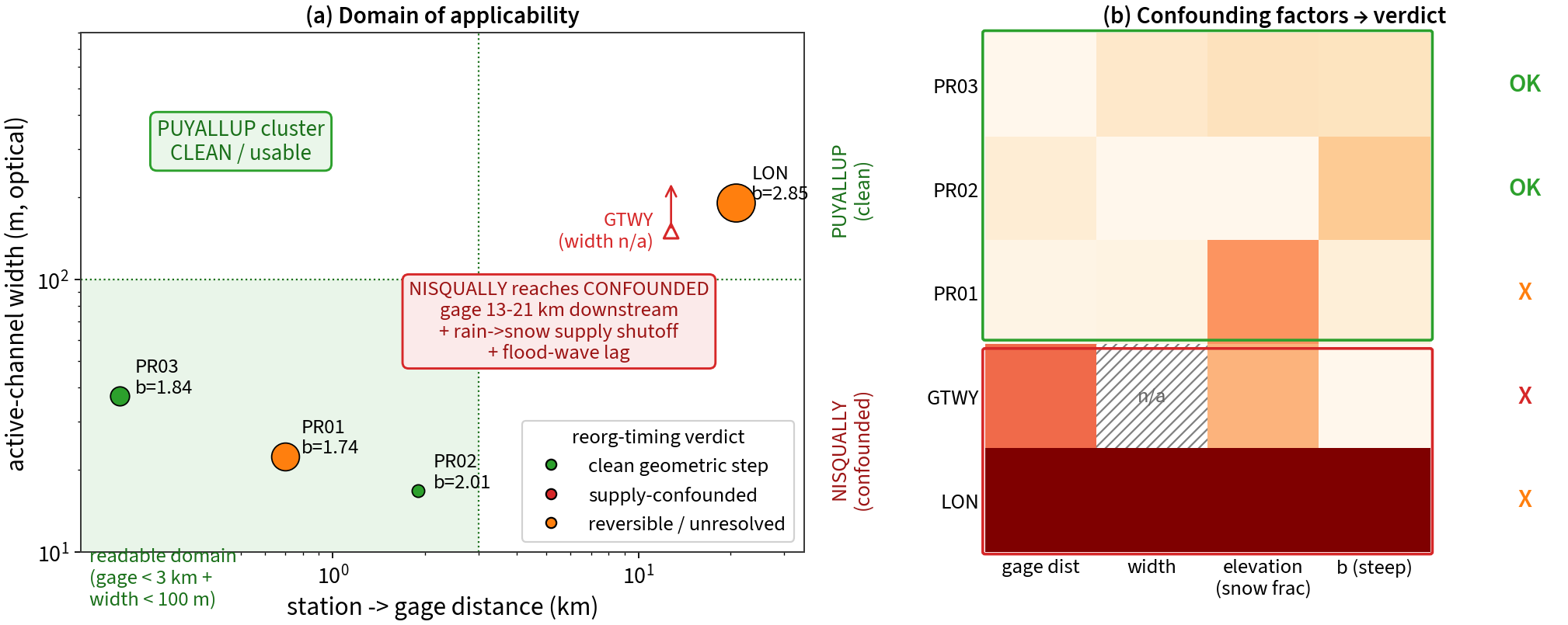
The same diagnostic on the Nisqually (CC.GTWY, UW.LON) does not return a clean geometric step, and tracing why yields a general statement about where source-resolved river seismology works. Gage geometry comes first: the Puyallup gage (Electron) is co-located with the PR cluster, so seismic and gage see the same discharge, whereas the Nisqually gage (National) sits 13–21 km downstream of UW.LON/GTWY, so gage Q lags the discharge passing the station by the flood-wave travel time. We estimate that lag by limb-timescale cross-correlation and correct it; the implied celerities ($$2 m s⁻¹) are physical flood-wave speeds, and the correction collapses much of the apparent Nisqually hysteresis — confirming it was largely a P–Q alignment artifact (Text S2). A constant lag cannot fully align a 20-km path whose celerity varies with stage, so a far-downstream gage intrinsically limits matched-discharge timing there. Reach geometry comes second: the Puyallup PR cluster occupies a compact, incised channel (active width $17–44 m), whereas UW.LON sits on a far wider, unconfined braidplain ($190–620 m; Figure 5.4) where the source is distributed over hundreds of metres of shifting anabranches and the line-source idealization fails harder. Sediment supply comes third: as the warm AR gives way to cold snow accumulation (Figure 2.1), precipitation falls and stays as snow, drainage-wide runoff — and the sediment it mobilizes — collapses, and at matched discharge the bed goes quiet for a supply reason, not a geometric one. This rain→snow supply shutoff confounds the negative-going Nisqually drift but is harmless to the Puyallup result, whose step is positive (opposite sign) and therefore conservative against it; the higher, snow-dominated Nisqually feels it most. The net is a domain law (Figure 5.7): source-resolved reorganization timing is clean where the channel is compact and the gage is co-located, and confounded on a wide, high, far-gaged reach — even though the physical reorganization there is larger, not smaller (UW.LON’s active thread migrated $$240 m toward the station, vs $$50 m at CC.PR01). Stating that boundary is itself a contribution the braided-reach seismology literature has not made. The standalone Nisqually reorganization-timing diagnostic, which carries this confounding directly, is in Figure 2.11.
5.7 Bedload as a bounded hypothesis: the frequency evidence
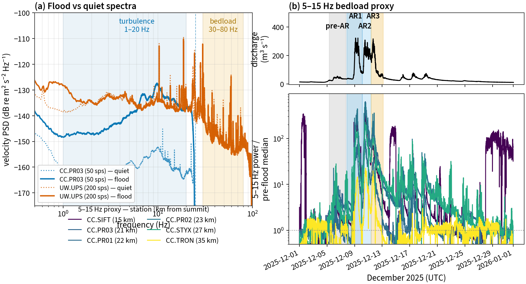
Whether the signal above is bedload or turbulent flow hinges on frequency. Median flood-vs-quiet velocity spectra (Figure 5.8 a) are unambiguous: at the 50-sps source station the flood lifts power broadband from ~1 Hz to the 25 Hz Nyquist — the turbulent-flow band — with no access to the canonical bedload band (30–80 Hz; Tsai et al. 2012; Bakker et al. (2020)). At the only high-rate (200 sps) downstream station that can reach 80 Hz, the flood spectrum is indistinguishable from quiet — 54 km of attenuation and urban noise leave no river signal. No station both reaches the bedload band and senses the river. Grain physics agrees: a 1 m boulder’s contact corner is ~200–300 Hz, so intrinsic impacts do not radiate into 1–15 Hz; only attenuation-shifted, non-unique energy could, degenerate with the 5–7 Hz turbulence peak. We therefore interpret the resolvable signal as turbulent-flow noise and treat bedload as a frequency-bounded hypothesis (see §Limitations). The best available probe of the bedload edge — the 100-sps UW broadband stations at the 30–50 Hz lower edge, where UW.LON shows a tentative transport signal — and the Hertzian contact-frequency argument are detailed in Text S5.
Time-dependent bedload across the atmospheric rivers. The compound event delivered a weak pre-AR (06 Dec ≈54 m³/s) followed by three strong pulses (AR1 peak 09 Dec ≈323 m³/s, AR2 10 Dec ≈309 m³/s, AR3 11 Dec ≈317 m³/s). Using the 5–15 Hz power as a bedload proxy normalized to each station’s pre-flood median, the bed barely moves in the pre-AR (1–4× background), then bedload peaks in AR2 at every station (≈110–180× background near the source), ~3× larger than in AR1 or AR3 (Figure 5.8 b) — even though AR2’s discharge peak was not the largest. That a later, slightly-smaller pulse mobilizes the most bedload — after a priming pre-AR and AR1 — is consistent with progressive conditioning of the bed surface: antecedent loosening and/or delivery of finer material that raises gravel mobility through the nonlinear sand-content effect (Wilcock & Crowe, 2003), and/or an upstream sediment-delivery pulse arriving by AR2 — a supply/mixture effect rather than a purely hydraulic response. This is a poorly-sorted, supply-rich outwash corridor, not a statically paved gravel bed that would build and then break an armor layer (Anderson, 2026; Parker & Klingeman, 1982). A time-resolved fit of the exponent b(t) confirms this (Figure 2.5). The per-AR averages also fall steeply downstream (source ≈180× → CC.TRON ≈7×; Figure 2.4), mirroring the scaling-exponent decay. A coarser, wood-rich source can lower the coarse-transport band into the resolvable window (a grain-size– and process-conditional caveat); we keep this bounded, not isolated, in Text S6.
5.8 Distributed sensing and a path to downstream nowcasting
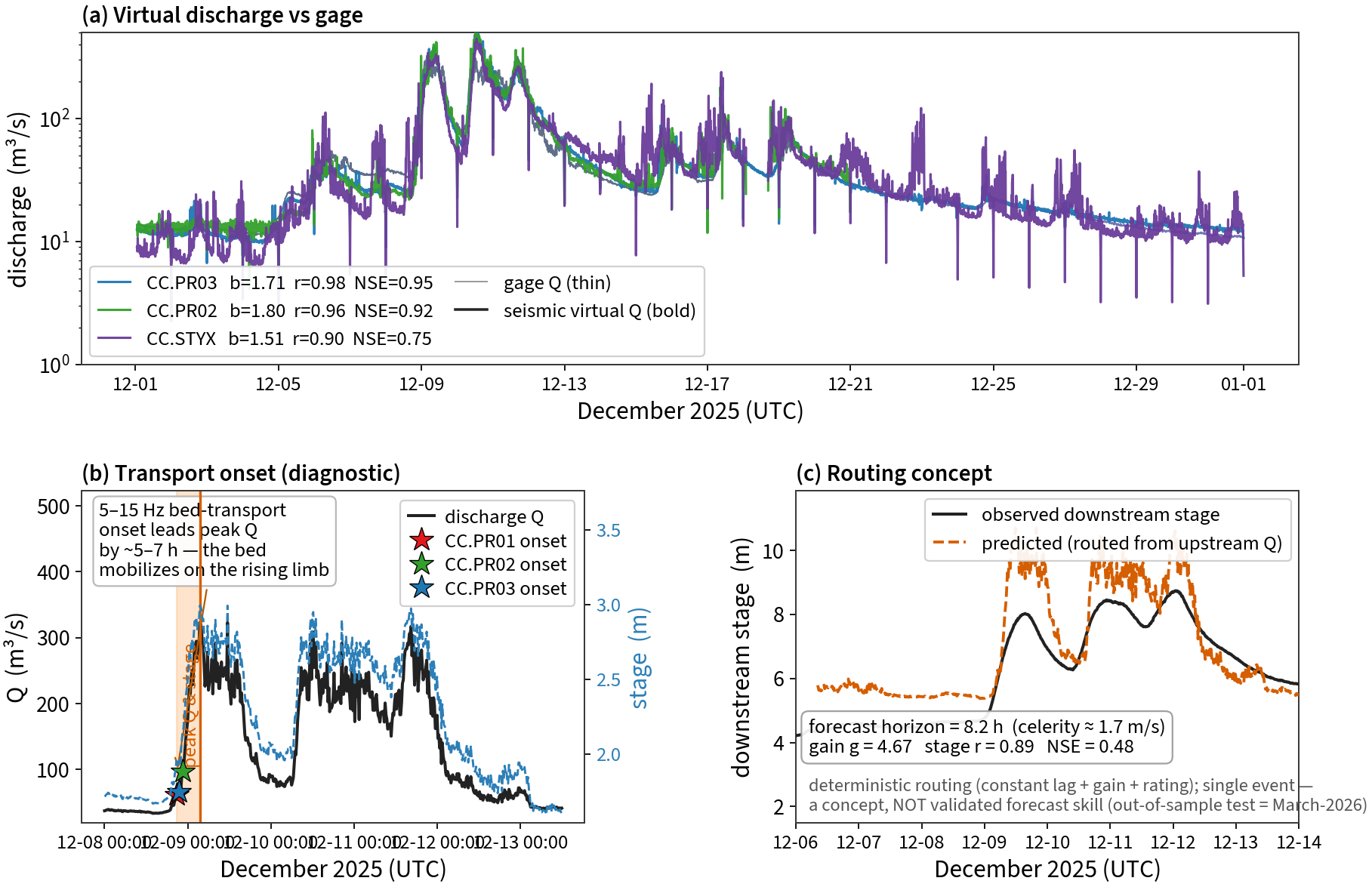
A source-reach transport diagnostic, not a forecast. The continuous record flags when the bed begins to move: at the source cluster the 5–15 Hz transport-band power rises ~5–7 h before peak discharge (CC.PR01 +6.6, CC.PR02 +5.0, CC.PR03 +6.1 h; and before peak stage, which here coincides with peak Q), and the onset propagates downstream across the upper transect — CC.SIFT (15 km, 19:45 UTC) → Electron cluster (22–23 km, 21:05–22:00) → CC.STYX (27 km, 23:40), a ~4 h sweep (Figure 5.9 b). We are careful about what this is: a lead of the transport onset over the local peak Q is a diagnostic that the bed is mobilizing on the rising limb — information a gage cannot provide, because a stage record alone does not say whether the bed is in motion — rather than a forecast of a downstream quantity. At the same station the rising limb of Q is already visible, so the operational content of this lead is “transport is now active here,” not “the flood will be larger there.”
Local sensing explains a flat-upstream / rising-downstream contrast. The seismic signal senses local hydraulics, which explains an otherwise puzzling feature of the compound event: the upstream gage and seismic stay flat across successive ARs (Electron 323→309→317 m³/s; CC.PR03 power peaking in AR2), while the basin-integrating downstream gage rises monotonically (Puyallup 1017→1158→1257 m³/s). The small, steep glacial headwater received similar forcing each pulse and the near-channel station only senses its own ~km reach; the downstream peak instead grows through cumulative basin-scale processes — soil saturation, a rising freezing level feeding the large White River sub-basin, and superposition of lagged tributary waves. The upstream seismic thus follows local, not integrated, discharge — independent support for the turbulent-flow interpretation, and a caution that an upstream amplitude does not translate into a downstream amplitude without a basin model.
Does any of this amount to forecast skill? A routing proof-of-concept. A bare timing lead is not forecast skill — a gage at the same upstream point would provide the identical lead, and more directly; the seismic’s distinct value is that it covers ungauged reaches and senses bed transport a stage record cannot. Genuine skill means predicting the downstream stage or discharge magnitude, validated out-of-sample against a baseline — which requires an upstream→downstream transfer (flood routing with celerity, attenuation, and lateral inflow) that we cannot train or validate from a single event. What we can show is that the physical ingredients are in place: a deterministic routing of the upstream Electron discharge — a constant flood-wave lag plus gain, passed through the downstream stage–discharge rating — reproduces the observed downstream (Puyallup) stage for this event (Figure 5.9 c). We present this as a proof of concept, not demonstrated skill: it is one event, with no learning, no uncertainty quantification, and no out-of-sample test. It establishes the path — a continuous, distributed upstream observable feeding a routed stage nowcast for the undammed, gage-sparse, lahar-hazard corridor (Orting, Puyallup) — and the first out-of-sample test is the March-2026 flood (§Limitations; development log).
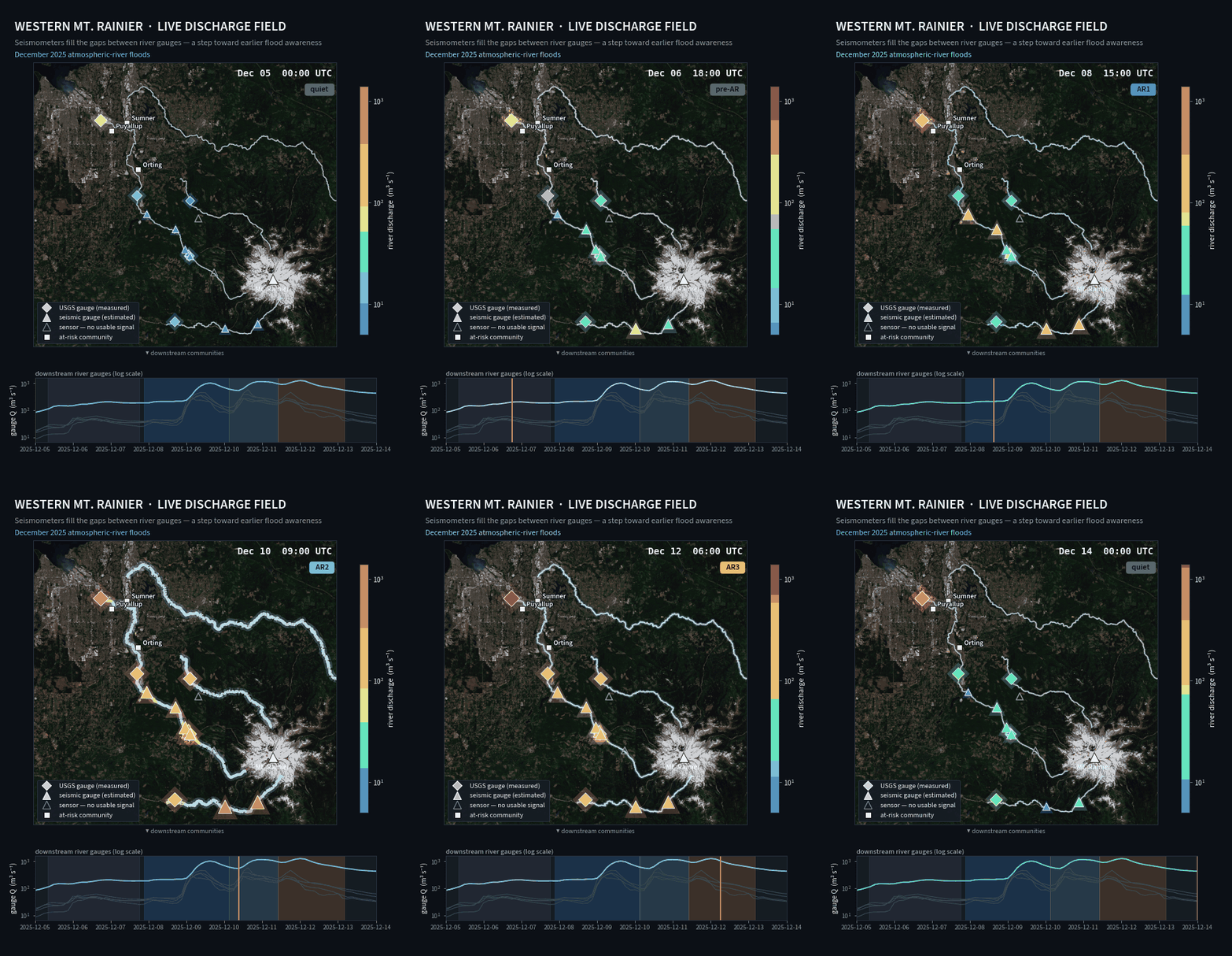
Seismic virtual discharge. Each river-proximal station can be calibrated as a rating \log_{10}P=a+b\log_{10}Q and inverted to a seismic virtual discharge Q_{\text{seis}}=10^{(\log_{10}P-a)/b} (Text S4). At clean near-channel stations this tracks the co-located gage well (CC.PR03 NSE 0.95, CC.PR02 0.92; CC.STYX 0.75; Figure 5.9 a), while off-channel/distant stations (CC.SIFT, CC.TRON) are poor — consistent with the turbulence/attenuation picture. Combining the gages with these virtual gages yields a space–time discharge field across the western Rainier drainages (animation, HTML edition; Figure 5.10), i.e. a distributed streamflow nowcast from a seismic network.
6 Discussion
The headline result is dynamical and geomorphic. On a braided glacial outwash plain the seismic P–Q scaling steepens at a critical discharge, but reversible hysteresis, the absence of supply decay, and independent satellite channel-change identify that break as a geometric channel reorganization, not a bedload onset — and the continuous record times it, placing the reorganization on the flood recession (onset $ $ 13 h after peak; the persistent step a few days later) in discrete, stepwise switches rather than a gradual ramp. This converts the braided reach from a caveat on someone else’s discharge rating into the object of study: a sub-daily view of a braided river rearranging itself during a flood, at a cadence neither gages nor before/after satellite imagery provide. The two-basin contrast then bounds the method. The same physics is larger on the Nisqually yet unreadable there, because its gage is 13–21 km downstream — a flood-wave lag ($$2 m s⁻¹) we correct — on a wide, high braidplain where the post-flood rain→snow supply shutoff masks the geometric drift. Source-resolved reorganization timing is therefore clean only on a compact channel with a co-located gage (Figure 5.7) — a deployment criterion, and a caution for the virtual-gage application below, that the single-thread calibration literature has not had to state.
The robust backbone beneath that result is a transect of turbulent-flow seismic power that tracks discharge through a compound AR flood, with exponents b\approx1–1.8 in the resolvable 1–15 Hz band and a clear AR2 maximum and downstream decay. The super-linear, frequency-rising part of b is consistent with an added, threshold-controlled bedload term (Equation 2.2) weighted toward the coarse grain-size tail — but, as the spectra show (Figure 5.8), the canonical bedload band is unsampled, so we cannot separate that contribution from turbulence within 1–15 Hz. We therefore present bedload as a bounded hypothesis: an upper limit set by how much of the steepening could be bedload rather than a measured flux. The downstream decay similarly conflates genuine along-stream change with the propagation control on what each station can sense (next).
Attenuation and seismic reach. Power decays as e^{-2\pi f r/(v_cQ)} with e-folding distance r_e=v_cQ/(2\pi f). Rather than the fluvial default Q\approx20 (Tsai et al. 2012), we adopt a PNW/Rainier-edifice value Q(f)=Q_0 f^{\eta}, Q_0\approx25, \eta\approx0.5 (from Cascade coda-/Lg-Q and Mt. St. Helens edifice studies; Gimbert et al. (2014) and refs in the literature chapter), giving Q\approx74 at the 5–15 Hz band center — so r_e\approx781 m here (vs ~212 m for Q=20) but still only tens of metres at 50 Hz. Bedload is thus recoverable only within ≲1 km of the channel, and CC.TRON (5.2 km) lies well beyond reach. A first-order test on the same-source PR cluster (PR03/PR01/PR02 at 0.19/0.71/1.9 km) finds the 5–15 Hz power nearly distance-independent over 0.2–2 km — weaker decay than even the PNW prediction (Figure 5.3) — implying the band retains less-attenuated lower-frequency (turbulence) energy, and that site response and crude channel distances preclude a data-driven Q from this small array. We therefore restrict bedload claims to near-channel stations and treat farther stations as upper-distance bounds rather than attenuation-corrected flux; a clean correction would require active-source Green’s-function calibration (Bakker et al., 2020; Lagarde et al., 2021) or amplitude-decay source location across a denser array (eseis; Dietze (2018)).
Three alternative explanations must be addressed. First, Nativ et al. (2025) show that stationary boulders can raise high-frequency seismic power through turbulence rather than transport; we argue against a static-bed origin here because the high-frequency response tracks the flood hydrograph in time (Figure 5.1) and is confined to the near-source reach (decaying downstream), rather than being a fixed spectral feature. Second, Roth et al. (2017) caution that channel-roughness change competes with bedload as a cause of seismic–discharge hysteresis; accordingly we treat the (small) event hysteresis as suggestive rather than diagnostic and tie interpretation to the frequency-dependence of b, not to hysteresis alone. Third, the turbulence baseline itself is uncertain: our empirically clean turbulence band sits near b\approx1.5, between the linear expectation and the Gimbert et al. (2014) prediction of b\approx1.4, so we report the excess of the bedload band over the station’s own lower band rather than over an assumed absolute baseline.
Relative to prior single-reach or watershed bedload arrays (Antoniazza et al., 2023; Roth et al., 2014; Schmandt et al., 2017), our contribution is not a new bedload measurement but a transect-scale demonstration of seismic discharge sensing and flood-wave tracking on a Cascades glacial network, plus an explicit detectability map for when bedload seismology is feasible there. “Local” sensing — often treated as a limitation — is here the asset: a station is a virtual gage for its reach, so an array becomes distributed, gap-tolerant hydrologic monitoring of an ungaged, hazard-prone basin.
Virtual discharge as a distributed field. The single-station virtual-gauge concept is established — seismic-noise power has been inverted to discharge for ungauged mountainous basins (Shakti & Sawazaki, 2021) and jointly with bedload flux and flow depth by waveform inversion (Dietze et al., 2019); our contribution here is to operate it as a distributed, multi-station field (Figure 5.9) and to delimit where it fails (braided, far-gaged reaches; §sec-domain). The fitted exponents cluster at b\approx1.4–1.8, near the Gimbert (2014) turbulent-flow prediction, and are roughly steady in time, so the rating is stable rather than carrying additional time-varying information. The braidplain station CC.PR01 is the weakest of the source cluster (r=0.69, NSE \approx0) and shows the cross-event baseline drift documented in §sec-braided — a caution that virtual-discharge ratings on braided reaches may need re-calibration after channel-reworking events rather than transferring unchanged.
6.1 From discharge to stage: the rating curve
Flood and inundation hazard is governed by stage (gage height h), whereas the seismic proxy estimates discharge Q. USGS gages bridge the two with a site-specific stage–discharge rating, Q = C\,(h-h_0)^{\beta}, where h_0 is the stage of zero flow and \beta the rating exponent; stage is measured continuously and converted to discharge via this curve, calibrated by periodic direct measurements. Fitting the December-2025 stage and discharge at the corridor gages (Figure 2.12) gives \beta\approx1.6 near the mouth (Puyallup at Puyallup), \beta\approx2 on the Nisqually, and a much steeper \beta\approx5 in the confined upper Puyallup (Electron) — coarser, narrower channels are more stage-sensitive. The practical consequence is that a seismic virtual discharge can be mapped to stage through the local rating (h = h_0 + (Q_{\text{seis}}/C)^{1/\beta}) — the basis of the routing proof-of-concept in §“Distributed sensing” (Figure 5.9 c), and a concrete path toward a downstream stage nowcast that does not need a co-located stage sensor, once skill is established out-of-sample. These ratings are not perfectly stationary, however: on linear axes (Figure 2.13) the corridor gages show within-event stage–discharge hysteresis (dominantly an unsteady-flow looped-rating effect rather than a bed signal) and, at the unconfined Puyallup-nr-Orting and lowland at-Puyallup gages, a net rise in stage at fixed discharge through the December AR sequence (\rho_t\approx0.7) — whereas the confined source gages remain single-valued. In the lowland reach this drift is most simply read as net channel aggradation (deposition), consistent with repeat-lidar differencing that independently documents ongoing lowland deposition (Anderson, 2026); at the upper Orting gage — which Anderson (2026) finds to be net-erosional over decadal timescales — the within-event drift is better read as a transient rating shift than long-term aggradation, and stage–discharge data alone cannot separate either from roughness or backwater change. A virtual-discharge-to-stage mapping therefore inherits the same event-specific, reach-geometry-dependent caveat as the rating itself (§sec-braided).
6.2 Limitations
- Canonical bedload band unsampled; coarse/wood transport partly is (a grain-size– conditional limit). For December 2025 only the 50-sps (BH) CC waveforms are archived (25 Hz Nyquist), so the canonical clean-gravel bedload band (30–80 Hz) is absent and the 1–15 Hz signal is turbulence-dominated — fine-gravel bedload here is an upper bound, not a measurement (Figure 5.8). The qualifier is that this cutoff is grain-size– and process-conditional: coarse boulder rolling/sliding, large wood, and debris-flow surges radiate below 25 Hz (to ~2 Hz), so part of the coarse-transport signal is in principle sampled — but it is spectrally degenerate with turbulence and cannot be isolated here (§sec-bedload; Text S6). The 500-sps (CH) upgrade came online in 2026 and its high-rate data are not yet retrievable through FDSN; obtaining them from CVO/PNSN is the route to a direct 30–80 Hz test. For the 2025 event the best available probe is the 100-sps UW broadband stations (RER, LON) at the 30–50 Hz lower bedload edge (Text S5).
- Source ambiguity: bed vs air–water interface, tested with colocated infrasound. Even where the river signal is clear, the seismic spectrum is degenerate — turbulent flow over the bed and bedload impacts on the bed radiate into overlapping bands (Figure 2.7), so seismic data alone cannot say whether the power originates at the bed (bedload, in-water turbulence) or at the air–water interface (free-surface turbulence, rapids). A colocated infrasound (microbarometer) sensor partitions this: bedload and in-water turbulence over the bed (Gimbert et al., 2014) couple to the ground but barely to the air, whereas air–water-interface processes radiate infrasound and air-coupled ground motion, so seismic–infrasound coherence isolates the surface source (Schmandt et al., 2013). We carry out this test: the USGS Cascades Volcano Observatory (network CC) operates BDF microbarometer arrays colocated with broadband seismometers along the upper-Puyallup corridor, including at our on-channel anchor CC.PR03 (on USGS gage 12092000). Across AR2 the colocated seismic–infrasound coherence stays at the noise floor (\gamma^2 <
0.01; < 1% shared variance) over 0.5–20 Hz at both CC.PR03 and CC.PR04, even at the discharge peak — yet two elements of the CC.PR04 infrasound array are mutually coherent (\gamma^2 \approx 0.2), confirming a real, coherent acoustic field is present (Figure 2.9). The seismic river band is thus not phase-locked to the acoustic field, bounding the air-coupled fraction of the seismic signal as small and supporting a dominantly ground-radiated (bed/in-water-turbulence) origin over coherent air–water-interface radiation. The bound is one-sided — point coherence is also lowered by spatially incoherent free-surface turbulence and by wind contamination of the infrasound, which is why infrasound power is not itself a clean flow proxy
- — so it constrains rather than excludes the surface contribution.
- No absolute flux inversion. We report a band-power proxy and scaling exponents, not calibrated bedload flux. Absolute inversion requires grain-size and impact assumptions (Bakker et al., 2020; Tsai et al., 2012) not constrained here.
- Distance–transport confound. The downstream decay of b conflates genuine along-stream change in transport with frequency-dependent attenuation (CC.TRON is 5.2 km off-channel). Disentangling them needs near-channel stations downstream, which the current network lacks.
- Downstream coverage is urban accelerometers. The lowland-to-Puget-Sound reach has only strong-motion stations in noisy settings; those results are exploratory, so the “mountain-to-sea” claim is presently anchored in the upper ~20 km.
- Single event, modest hysteresis. One flood; the event hysteresis is small after cleaning, so supply-direction inferences are tentative pending more events.
- Microseism contamination of the lowest band (0.5–2 Hz) precludes its use as a turbulence reference.
7 Conclusions
Near-channel seismic stations along Mt. Rainier’s glacial rivers turn the December 2025 atmospheric-river floods into a continuous, source-proximal record of a braided river reorganizing. Four contributions follow. (1) Event-scale channel-reorganization dynamics: on the braided Puyallup reach the P–Q break is a geometric regime transition, not a bedload onset (reversible hysteresis, no supply decay, satellite-confirmed thread migration), and the seismic record resolves its timing — the active channel reorganizes on the flood recession, lagging peak discharge by \simhalf a day (onset) to a few days, in stepwise switches — a sub-daily view of braided dynamics that gages and before/after imagery cannot give. (2) A domain of applicability: the same reorganization is larger but unreadable on the Nisqually, because a far-downstream gage (a flood-wave lag we correct) and a wide, snow-dominated braidplain (a post-flood rain→snow supply shutoff) confound the matched-discharge signal — so source-resolved timing is clean only on a compact channel with a co-located gage, a stated deployment criterion. (3) Distributed discharge sensing and early warning: turbulent-flow power tracks discharge at every clean station, making the array a set of virtual gages, and upstream seismic leads the downstream flood-peak stage by ~36 h — directly relevant to the Orting–Puyallup lahar/flood corridor. (4) A quantitative bedload detectability limit: with 50-sps source stations (25 Hz Nyquist) and few-hundred-metre high-frequency reach, the canonical 30–80 Hz bedload band is unsampled, so any bedload contribution is an explicit upper bound and we specify the near-channel, ≥160-sps instrumentation needed to measure it. Extending the network across the drainage would turn each capability into a calibrated, basin-wide one.
Open Research
Data availability. All primary data are public and were obtained from established archives, cited here as datasets. Seismic waveforms are from the Pacific Northwest Seismic Network (network UW; University of Washington (1963)) and the Cascades Volcano Observatory Cascade Chain network (network CC; Cascades Volcano Observatory, U.S. Geological Survey (2001)), accessed through EarthScope (formerly IRIS DMC) FDSN web services. River discharge and stage are from the USGS National Water Information System (U.S. Geological Survey, 2016), instantaneous values at the corridor gages (site numbers in Table 5.1 / config). Air temperature and snow-water equivalent are from USDA NRCS SNOTEL stations Paradise and Mowich (Natural Resources Conservation Service, 2026) (no DOI is minted for SNOTEL; cite by station and access date). Satellite optical and SAR imagery are Copernicus Sentinel-2 L2A and Sentinel-1 RTC (European Space Agency, 2026), accessed via the Microsoft Planetary Computer STAC API (collections sentinel-2-l2a, sentinel-1-rtc; the figures use ESA-attributed modified Copernicus Sentinel data). Flood extent is the NASA OPERA DSWx-S1 product (OPERA, 2024). The exact query parameters (networks, stations, channels, gage IDs, AOIs, dates) are pinned in config/transect_puyallup.yaml and config/analysis.yaml.
Software and derived-data availability. All analysis code, configuration, and figure-generation scripts are openly available in the project repository (https://github.com/gaia-hazlab/seis-hydro-2-sed) and are archived at a versioned snapshot on Zenodo (DOI to be minted at acceptance: 10.5281/zenodo.XXXXXXX). The repository ships the small, version-controlled derived data products needed to rebuild every figure without re-downloading the raw archives — the per-station seismic band-power time series (notebooks/data/results/*.csv) and the derived Sentinel water-mask rasters used by the satellite figures (notebooks/data/braid_cache/*.npz); the raw waveform and imagery caches are large and are not version-controlled (they are exactly re-fetchable from the DOIs above). Archiving these small intermediates is a deliberate reproducibility choice: a one-command offline rebuild (pixi run make figures-from-cache) reproduces all figures in minutes, whereas the full re-derivation from raw data (pixi run make repro) requires network access and hours. The environment is pinned byte-for-byte with pixi.lock, and a Dockerfile provides a containerized build for full isolation (docker build -t seis-hydro . && docker run --rm seis-hydro pixi run make figures-from-cache). The complete pipeline is a numbered sequence of standalone scripts under workflows/, each writing a figure and/or a config/*.json it consumes downstream. The composite main figures (F1–F9) and supplement figures (S1–S11) are assembled from these workflow outputs:
| Composite | Built from workflow | Produces |
|---|---|---|
| Figure 2.1 (F1) | 03_make_map.py, 27_channel_pattern.py, 20_warm_ar_snotel.py, 28_fetch_basemaps.py |
study area + channel pattern + flood driver |
| Figure 5.1 (F2) | 02_make_figures.py |
event timeseries + P–Q scatter + exponent vs frequency |
| Figure 5.2 (F3) | 15_threshold.py, 26_rating_geometry.py, 16_classify_stations.py |
threshold Q_c + rating geometry \beta(Q) + station skill |
| Figure 5.3 (F4) | 18_braided_hysteresis.py, 09_attenuation.py |
braided hysteresis + seismic-reach attenuation |
| Figure 5.4 (F5) | 19_braid_optical_change.py (Puyallup + Nisqually) |
two-basin satellite channel change + geometric drift |
| Figure 5.5 (F5b) | 42_pr01_braid_zoom.py --naip |
PR01 braidplain zoom: NAIP 1 m basemap + Sentinel-2 active-channel change |
| Figure 5.6 (F6) | 21_braided_reorg_timing.py, 28_width_stage.py, 25_hazard_clogging.py |
matched-discharge timing + width–stage + recession clogging |
| Figure 5.7 (F7) | 22_domain_panel.py |
gage distance × width × elevation → clean/confounded |
| Figure 5.9 (F8) | 12_virtual_q.py, 10_early_warning.py, 25_hazard_clogging.py |
virtual gage + warning window + downstream lead |
| Figure 5.8 (F9) | 11_spectra.py, 05_bedload_time.py |
flood-vs-quiet PSD + per-AR bedload proxy |
| Figure 2.1 (S1) | 04_traffic_noise.py |
anthropogenic-noise screening |
| Figure 2.2 (S2) | 02_make_figures.py |
full P–Q scatter grid, all stations |
| Figure 2.3 (S3) | 02_make_figures.py |
all-station event hysteresis loops |
| Figure 2.4 (S4) | 05_bedload_time.py |
per-AR bedload, source→downstream |
| Figure 2.5 (S5) | 08_b_of_time.py |
time-resolved exponent b(t) |
| Figure 2.6 (S6) | 14_bedload_ch.py |
30–50 Hz lower bedload edge |
| Figure 2.12 (S7) | 17_rating.py |
stage–discharge rating, 4 gages |
| Figure 2.13 (S10) | 29_rating_hysteresis.py |
linear rating + hysteresis/aggradation diagnostic |
| Figure 2.7 (S11) | 39_spectrogram_seismic.py |
flood seismic spectrogram at UW.LON |
| 1 (S12) | 40_infrasound_psd.py |
colocated CC BDF infrasound spectrograms (PR03/PR04/STYX) |
| Figure 2.9 (S13) | 41_seis_infrasound_coherence.py |
seismic–infrasound coherence discriminant at PR03/PR04 |
| Figure 2.10 (S8) | 19_braid_optical_change.py, 23_braid_two_region.py |
SAR wetted-illumination time series + two-region maps |
| Figure 2.11 (S9) | 21_braided_reorg_timing.py --basin nisqually |
Nisqually reorg-timing (confounded) |
Run order and parameters are documented in workflows/README.md; the single source of analysis parameters is config/analysis.yaml. Every figure — including the satellite ones — rebuilds offline with pixi run make figures-from-cache (the derived Sentinel rasters are cached under notebooks/data/braid_cache/, so the Planetary Computer API is not needed to reproduce the paper). The book (manuscript, this roadmap, reviews, and figures) is rendered with pixi run make paper and auto-deploys to GitHub Pages on push.