import rioxarray as rxr
import xarray as xr
import xvec
import os
import geopandas as gpd
import pandas as pd
import xyzservices
import numpy as np
from zarr.storage import ObjectStore
from obstore.store import S3Store
import matplotlib.pyplot as plt
# %config InlineBackend.figure_format = 'retina'
# %matplotlib inlinegeojson = "https://raw.githubusercontent.com/DSHydro/skagit-met/refs/heads/main/data/GIS/SkagitBoundary.json"
# The CLI reads -s 2025-12-01 -e 2025-12-16 as these UTC bounds (a date-only end includes the day).
# Staging reads one day beyond each end, so the store holds more; the analysis below uses [start, end].
start = "2025-12-01T00:00:00"
end = "2025-12-16T23:59:59"
# -o is a folder: skagit/skagit.zarr, its STAC Item skagit/skagit.json and skagit/stage.yaml
output = "s3://gaia/scratch/public/skagit"
store = f"{output}/skagit.zarr"
# gaia align -o is a folder too: skagit-aligned/skagit-aligned.zarr and skagit-aligned/skagit-aligned.json
aligned = "s3://gaia/scratch/public/skagit-aligned"Stage data on S3 via CLI
Note: I’m writing this under a ‘scratch’ prefix that automatically deletes after 2 weeks
# Run CLI
!gaia stage --config conus-precip -i {geojson} -s {start} -e {end} --output {output} --overwrite
11:43:38 [ 1.3s] stagefile: Wrote s3://gaia/scratch/public/skagit/stage.yaml
11:43:38 [ 1.3s] runner: synoptic: loading (2025-12-01T00:00:00/2025-12-16T23:59:59, read as 2025-11-30T00:00:00/2025-12-17T23:59:59)
11:43:38 [ 1.3s] datasets.synoptic: querying station metadata from https://api.synopticdata.com/v2
11:43:38 [   1.4s] datasets.synoptic: found 23 stations with precip_accum in the AOI
11:43:38 [   1.4s] datasets.synoptic: fetching timeseries for 23 station(s)
11:43:39 [ 2.2s] io: Writing Zarr to s3://gaia/scratch/public/skagit/skagit.zarr
11:43:43 [ 6.2s] io: Saved s3://gaia/scratch/public/skagit/skagit.zarr
11:43:43 [   6.3s] io: Wrote STAC item s3://gaia/scratch/public/skagit/skagit.json
11:43:43 [   6.3s] runner: prism: loading (2025-12-01T00:00:00/2025-12-16T23:59:59, read as 2025-11-30T00:00:00/2025-12-17T23:59:59)
11:43:43 [ 6.5s] prism_cache.cache: PRISM ppt: 18 of 18 grid(s) in cache https://s3.kopah.uw.edu/gaia/public/prism (0 provisional, 0 missing)
11:43:44 [ 6.6s] datasets.prism: PRISM ppt: reading 18 day(s) x 164 x 208 cells from cached COGs
11:43:49 [ 12.6s] io: Writing Zarr to s3://gaia/scratch/public/skagit/skagit.zarr
11:43:54 [ 17.5s] io: Saved s3://gaia/scratch/public/skagit/skagit.zarr
11:43:55 [  17.8s] io: Wrote STAC item s3://gaia/scratch/public/skagit/skagit.json
11:43:55 [  17.8s] runner: hrrr: loading (2025-12-01T00:00:00/2025-12-16T23:59:59, read as 2025-11-30T00:00:00/2025-12-17T23:59:59)
11:43:55 [  17.8s] datasets.hrrr: opening dynamical.org Icechunk repo s3://dynamical-noaa-hrrr/noaa-hrrr-analysis/v0.2.0.icechunk/
11:43:56 [ 19.2s] datasets.hrrr: HRRR precipitation_surface: reading 432 hour(s) x 50 x 47 cells (2025-11-30T00:00 to 2025-12-17T23:00)
11:43:58 [ 20.6s] io: Writing Zarr to s3://gaia/scratch/public/skagit/skagit.zarr
11:44:04 [ 27.1s] io: Saved s3://gaia/scratch/public/skagit/skagit.zarr
11:44:04 [  27.3s] io: Wrote STAC item s3://gaia/scratch/public/skagit/skagit.json
11:44:04 [  27.3s] runner: Done
# Check that it's there!
!aws s3 ls {output}/
PRE skagit.zarr/
2026-10-21 11:44:04 3560 skagit.json
2026-10-21 11:43:38 656 stage.yaml
Work with staged data
Our bucket has anonymous read access, so anyone can access it
# Kopah (Ceph) S3 access. obstore needs the endpoint explicitly, and path-style requests.
# Anything under scratch/public/ is anonymously readable, so no credentials needed
s3gaia_test = S3Store(
    bucket="gaia",
    prefix="scratch/public/skagit/skagit.zarr",
    endpoint="https://s3.kopah.uw.edu",
    region="us-west-2",  # not actually used with kopah
    virtual_hosted_style_request=False,
    skip_signature=True, # anonymous read-only access
)

# Zarr-aware handler for reading from S3
gaia_zarr_store = ObjectStore(s3gaia_test, read_only=True)
dt = xr.open_datatree(gaia_zarr_store, engine="zarr", zarr_format=3, consolidated=False)
dt.groups('/',
'/stations',
'/rasters',
'/stations/synoptic',
'/rasters/hrrr',
'/rasters/prism')Weather station timeseries
from gaia_cli import stations

# The store keeps every station report (a CF ragged array, see dev/stations.md)
DS_reports = xr.open_dataset(
    gaia_zarr_store,
    engine="zarr",
    zarr_format=3,
    consolidated=True,
    group="stations/synoptic",
)
# Hourly grid: each hour holds the latest report at or before it (precipitation_report_time)
DS_stations = stations.to_grid(DS_reports)
DS_stations# Reduce to single time step for GeoPandas
gf = DS_stations.max(dim="time").xvec.to_geopandas()
gf.head()aoi = gpd.read_file(geojson)
# Basmap must be set on first map call
basemap = xyzservices.providers.Esri.WorldTerrain # or WorldImagery
m = aoi.explore(style_kwds={"color": "magenta", "fill": False}, tiles=basemap)
gf.explore(
m=m, column="precipitation", popup=True, tooltip="station"
) # , cmap='Blues', marker_kwds={'radius': 8})DA = DS_stations["precipitation"]
fig, ax = plt.subplots()
DA.plot(ax=ax, x="time", hue="station")
legend = plt.gca().get_legend()
# legend.set_bbox_to_anchor((1.05, 1))
plt.setp(legend.get_texts(), fontsize=8)
legend.set_loc("upper left")
plt.title("Skagit Basin Accumulated Precipitation Time Series by Station")
plt.ylabel("Precipitation (mm)");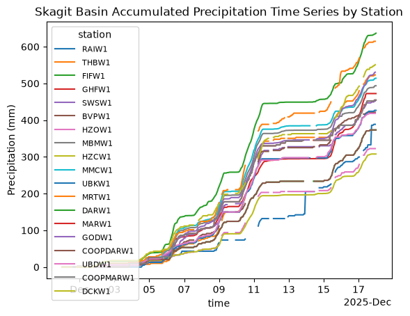
# Map view
# TODO: add station label annotations
fig, ax = DA.max(dim="time").xvec.plot()
aoi.plot(ax=ax, color="none", edgecolor="magenta");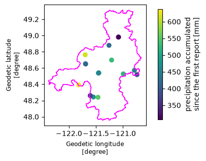
Raster data: PRISM and HRRR
# The rasters group has one child per product (prism, hrrr), each on its native grid.
# zarr_format=3 skips probing for v2 metadata (missing keys return 403, not 404, for anonymous reads)
DT = xr.open_datatree(
    gaia_zarr_store,
    engine="zarr",
    zarr_format=3,
    consolidated=True,
    group="rasters",
)
DT1. Native (unaligned) grids
gaia stage keeps each raster on the grid and time step of its source (see dev/prism.md, dev/hrrr.md):
| PRISM | HRRR | |
|---|---|---|
| CRS | EPSG:4269 (lat/lon), ~800 m | Lambert Conformal, 3 km |
| Time step | daily; date D covers (D−1 12:00, D 12:00] UTC | hourly; time T covers (T−1 h, T] |
time_bounds records the interval each value covers. Working on native grids means doing any alignment yourself, but it is the most faithful way to compare against stations, because no regridding happens.
prism = DT["prism"].to_dataset()
hrrr = DT["hrrr"].to_dataset()

for name, ds in [("PRISM", prism), ("HRRR", hrrr)]:
    crs = ds.rio.crs
    first = [str(t)[:16] for t in ds.time_bounds.values[0]]
    print(
        f"{name}: CRS {crs.to_epsg() or 'custom (Lambert Conformal)'}, "
        f"resolution {tuple(round(abs(r), 4) for r in ds.rio.resolution())}, "
        f"{ds.sizes['time']} time steps, first covers {first}"
    )

# PRISM covers the conterminous US only: the Skagit headwaters north of 49°N (British Columbia)
# have no PRISM data. Basin means below use the US part of the AOI so both products cover the same area.
from shapely.geometry import box

aoi_us = aoi.clip(box(-180, 0, 180, 49.0))
share = aoi_us.to_crs("EPSG:5070").area.sum() / aoi.to_crs("EPSG:5070").area.sum()
print(f"US share of the AOI: {share:.0%}")
PRISM: CRS 4269, resolution (0.0083, 0.0083), 18 time steps, first covers ['2025-11-29T12:00', '2025-11-30T12:00']
HRRR: CRS custom (Lambert Conformal), resolution (3000.0, 3000.0), 432 time steps, first covers ['2025-11-29T23:00', '2025-11-30T00:00']
US share of the AOI: 87%
A common accumulation window. Station values are running accumulations, PRISM days end at 12 UTC, and HRRR hours end on the hour. The store holds a day more on each side than requested, so align.common_window picks the longest interval inside [start, end] made of whole PRISM days and HRRR hours. align.select_window keeps each raster’s time steps inside it, and the station accumulations are differenced over exactly the same interval.
from gaia_cli import align

# The longest interval inside [start, end] made of whole PRISM days and HRRR hours
t0, t1 = align.common_window(DT, start, end)
prism_w = align.select_window(prism, t0, t1)
hrrr_w = align.select_window(hrrr, t0, t1)

prism_total = prism_w.precipitation.sum("time", min_count=1)
hrrr_total = hrrr_w.precipitation.sum("time", min_count=1)
station_total = DS_stations.precipitation.sel(time=t1) - DS_stations.precipitation.sel(time=t0)

window = f"{t0:%Y-%m-%d %H:%M} to {t1:%Y-%m-%d %H:%M} UTC"
print(f"Window {window}: {prism_w.sizes['time']} PRISM days, {hrrr_w.sizes['time']} HRRR hours")
Window 2025-12-01 12:00 to 2025-12-16 12:00 UTC: 15 PRISM days, 360 HRRR hours
COLORS = {"PRISM": "#2a78d6", "HRRR": "#eb6834"}  # fixed identity colors for the whole notebook

vmax = float(max(prism_total.max(), hrrr_total.max()))
fig, axes = plt.subplots(1, 2, figsize=(12, 5), layout="constrained")
panels = [("PRISM: 800 m, EPSG:4269", prism_total), ("HRRR: 3 km, Lambert Conformal", hrrr_total)]
for ax, (title, total) in zip(axes, panels):
    crs = total.rio.crs
    im = total.plot.imshow(ax=ax, cmap="Blues", vmin=0, vmax=vmax, add_colorbar=False)
    aoi.to_crs(crs).plot(ax=ax, facecolor="none", edgecolor="k", linewidth=0.8)
    xy = gpd.GeoSeries(DS_stations.geometry.values, crs="EPSG:4326").to_crs(crs)
    ax.scatter(xy.x, xy.y, c=station_total, cmap="Blues", vmin=0, vmax=vmax,
               s=60, edgecolor="k", linewidth=0.6)
    # degrees are not square on the ground; scale lon by cos(lat) for geographic grids
    ax.set_aspect(1 / np.cos(np.deg2rad(48.5)) if crs.is_geographic else "equal")
    ax.set_title(title)
    ax.xaxis.set_major_locator(plt.MaxNLocator(4))
fig.colorbar(im, ax=axes, label="Precipitation (mm)", shrink=0.9)
fig.suptitle(f"Event totals on native grids, {window}\n(circles: stations, same color scale)");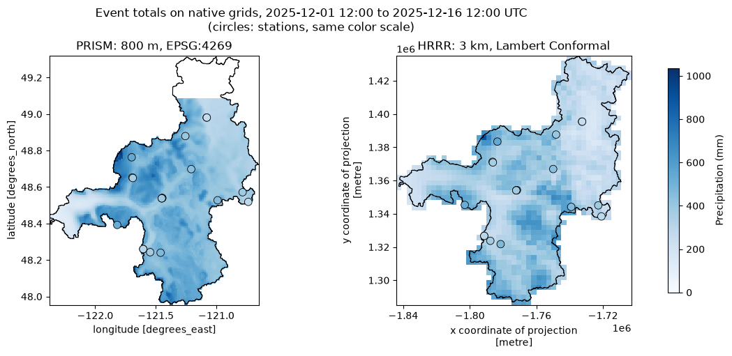
☝️ Note that PRISM does not extend into Canada unfortunately.
Stations vs. native rasters
Sample each raster at the station locations (nearest cell, no regridding). The station points are reprojected into each raster’s CRS first.
def sample(total, geoms):
    pts = gpd.GeoSeries(geoms, crs="EPSG:4326").to_crs(total.rio.crs)
    return total.xvec.extract_points(
        pts.values, x_coords="x", y_coords="y", crs=total.rio.crs
    ).values


df = pd.DataFrame(
    {
        "station": DS_stations.station.values,
        "elevation_m": DS_stations.elevation.values,
        "observed": station_total.values,
        "PRISM": sample(prism_total, DS_stations.geometry.values),
        "HRRR": sample(hrrr_total, DS_stations.geometry.values),
    }
).dropna()

err = {p: df[p] - df.observed for p in COLORS}
summary = pd.DataFrame(
    {
        p: {
            "mean error (mm)": e.mean(),
            "bias (%)": 100 * e.sum() / df.observed.sum(),
            "RMSE (mm)": np.sqrt((e**2).mean()),
            "correlation": df[p].corr(df.observed),
        }
        for p, e in err.items()
    }
).T.round(2)
print(f"{len(df)} stations with complete records over {window}")
summary
19 stations with complete records over 2025-12-01 12:00 to 2025-12-16 12:00 UTC
fig, ax = plt.subplots(figsize=(5.5, 5.5), layout="constrained")
lim = 1.05 * df[["observed", *COLORS]].max().max()
ax.plot([0, lim], [0, lim], color="0.6", lw=1, zorder=0)
ax.annotate("1:1", (0.95 * lim, 0.9 * lim), ha="left", va="top", color="0.4", fontsize=9)
for name, color in COLORS.items():
    ax.scatter(df.observed, df[name], s=50, color=color, edgecolor="white", linewidth=1.5, label=name)
ax.set(
    xlim=(0, lim), ylim=(0, lim), aspect="equal",
    xlabel="Station total (mm)", ylabel="Raster total at station (mm)",
    title=f"Stations vs. native rasters\n{window}",
)
ax.grid(alpha=0.3)
ax.legend(frameon=False, loc="upper left");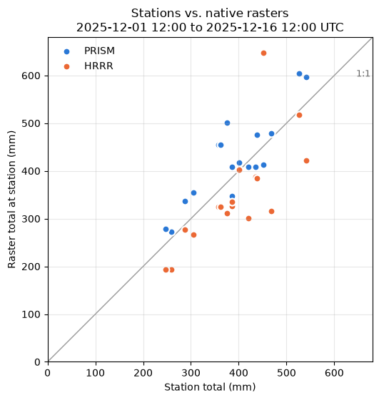
Basin-mean accumulation at native time steps
The exact area-weighted mean over the US part of the AOI polygon (xvec + exactextract) of each native grid, accumulated over time. Each PRISM value is plotted at the end of its day (12 UTC), where it lines up with HRRR’s hour-ending values. Both curves cover the window above.
def basin_mean(da):
    da = da.drop_vars([c for c in ("latitude", "longitude") if c in da.coords])
    geom = aoi_us.to_crs(da.rio.crs).geometry
    zs = da.xvec.zonal_stats(geom, x_coords="x", y_coords="y", stats="mean", method="exactextract")
    return zs.isel(geometry=0)


# The same window as above
prism_cum = basin_mean(prism_w.precipitation).cumsum("time")
prism_cum = prism_cum.assign_coords(time=prism_w.time_bounds.values[:, 1])  # day ends
hrrr_cum = basin_mean(hrrr_w.precipitation).cumsum("time")  # time is the hour end

fig, ax = plt.subplots(figsize=(10, 4), layout="constrained")
ax.plot(hrrr_cum.time, hrrr_cum, color=COLORS["HRRR"], lw=2, label="HRRR (hourly)")
ax.plot(prism_cum.time, prism_cum, color=COLORS["PRISM"], lw=2, marker="o", ms=8,
        markeredgecolor="white", label="PRISM (daily, at 12 UTC)")
for name, cum in [("PRISM", prism_cum), ("HRRR", hrrr_cum)]:
    ax.annotate(f"{float(cum[-1]):.0f} mm", (cum.time.values[-1], float(cum[-1])),
                xytext=(6, 0), textcoords="offset points", va="center", fontsize=9)
ax.set(ylabel="Basin-mean accumulation (mm)", title="Skagit basin (US part), native time steps")
ax.grid(alpha=0.3)
ax.legend(frameon=False, loc="upper left");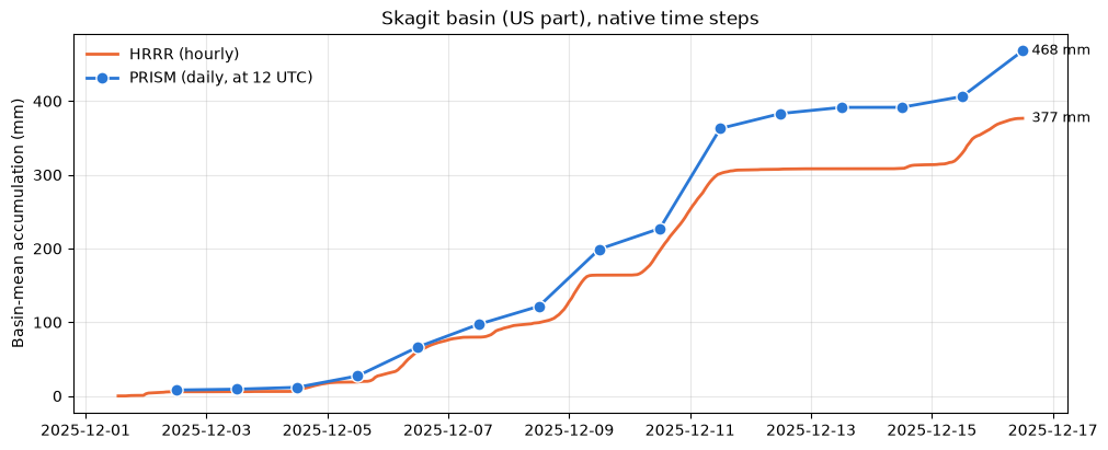
2. Aligned grids
gaia align puts the rasters on one grid and one time step. By default it sums HRRR’s hours into PRISM days (the coarsest time step), then regrids PRISM once, area-weighted (conservative), onto HRRR’s 3 km grid (the coarsest grid). It writes a new store and leaves the native one untouched (see dev/reprojecting.md). These aligned datacubes are much easier to work with, but opinionated choices have been made about how to align the rasters, so you may want to do your own alignment if you have a different idea!
!gaia align -i {store} -o {aligned} --aoi {geojson} --overwrite11:44:18 [ 2.2s] align: time target rasters/prism (18 step(s))
11:44:22 [ 5.9s] align: grid target rasters/hrrr (50 x 47 cells)
11:44:22 [ 6.3s] align: regridding rasters/prism/precipitation (conservative)
11:44:29 [ 13.2s] io: Writing Zarr to s3://gaia/scratch/public/skagit-aligned/skagit-aligned.zarr
11:44:38 [ 22.4s] io: Saved s3://gaia/scratch/public/skagit-aligned/skagit-aligned.zarr
11:44:38 [ 22.6s] io: Wrote STAC item s3://gaia/scratch/public/skagit-aligned/skagit-aligned.json
11:44:38 [ 22.6s] align: Done
s3gaia_test = S3Store(
    bucket="gaia",
    prefix="scratch/public/skagit-aligned/skagit-aligned.zarr",
    endpoint="https://s3.kopah.uw.edu",
    region="us-west-2",  # not actually used with kopah
    virtual_hosted_style_request=False,
    skip_signature=True, # anonymous read-only access
)

# Zarr-aware handler for reading from S3
gaia_zarr_store = ObjectStore(s3gaia_test, read_only=True)

DTa = xr.open_datatree(
    gaia_zarr_store,
    engine="zarr",
    zarr_format=3,
    consolidated=True,
    group="rasters",
)
DTa# The same window as for the native grids
pa = align.select_window(DTa["prism"].to_dataset(), t0, t1).precipitation
ha = align.select_window(DTa["hrrr"].to_dataset(), t0, t1).precipitation
# PRISM has no data north of 49°N (British Columbia); compare only cells where both products have data
both = pa.notnull() & ha.notnull()
pa, ha = pa.where(both), ha.where(both)
# Same grid and time steps now, so the products can be compared cell by cell
assert pa.x.equals(ha.x) and pa.y.equals(ha.y) and pa.time.equals(ha.time)
print(f"{dict(pa.sizes)}; PRISM regridded with {pa.attrs['regrid_method']!r}; HRRR {ha.attrs['aggregated_from']} per day"){'time': 15, 'y': 50, 'x': 47}; PRISM regridded with 'conservative'; HRRR 24 values of 60 minutes per day
prism_tot = pa.sum("time", min_count=1)
hrrr_tot = ha.sum("time", min_count=1)
diff = hrrr_tot - prism_tot

vmax = float(max(prism_tot.max(), hrrr_tot.max()))
dmax = float(abs(diff).max())
aoi_grid = aoi.to_crs(ha.rio.crs)

fig, axes = plt.subplots(1, 3, figsize=(16, 5), layout="constrained", sharex=True, sharey=True)
for ax, total, title in [(axes[0], prism_tot, "PRISM (regridded to 3 km)"), (axes[1], hrrr_tot, "HRRR")]:
    im = total.plot.imshow(ax=ax, cmap="Blues", vmin=0, vmax=vmax, add_colorbar=False)
    ax.set_title(title)
fig.colorbar(im, ax=axes[:2], label="Event total (mm)", shrink=0.9)

# Diverging: blue = HRRR wetter, red = HRRR drier, light midpoint = agreement
im_d = diff.plot.imshow(ax=axes[2], cmap="RdBu", vmin=-dmax, vmax=dmax, add_colorbar=False)
fig.colorbar(im_d, ax=axes[2], label="HRRR − PRISM (mm)", shrink=0.9)
axes[2].set_title("HRRR − PRISM (blue: HRRR wetter)")

for ax in axes:
    aoi_grid.plot(ax=ax, facecolor="none", edgecolor="k", linewidth=0.8)
    ax.set_aspect("equal")
    ax.set(xlabel="x (m)", ylabel="y (m)")
fig.suptitle(f"Aligned 3 km grid, event totals {window}");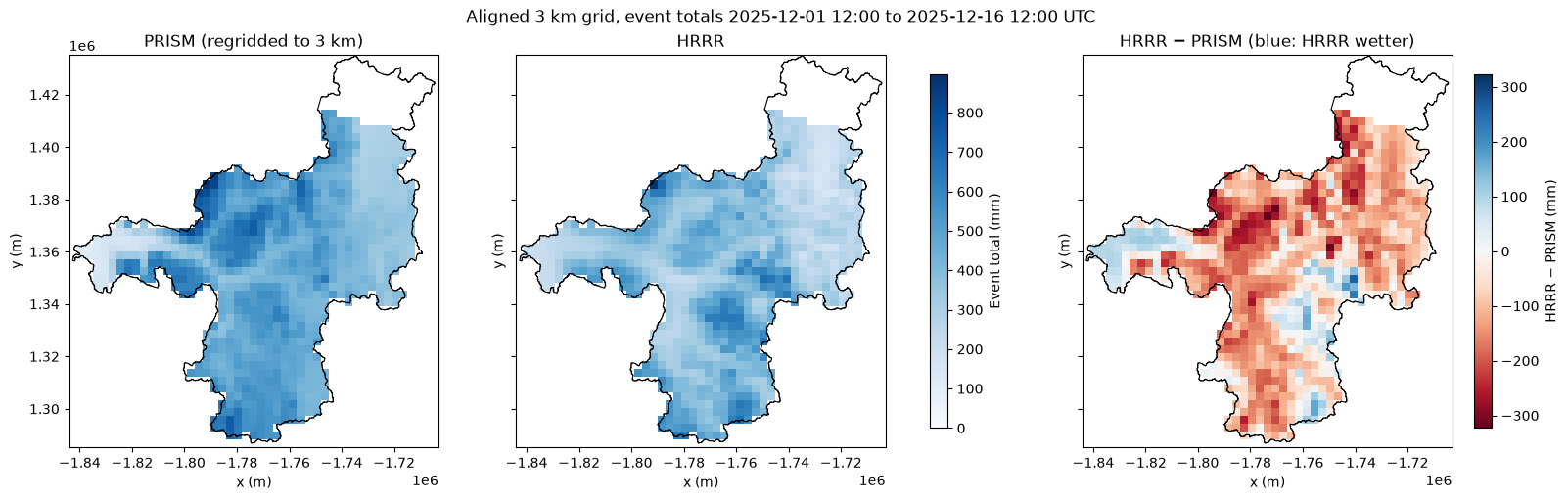
daily = pd.DataFrame({name: da.mean(["x", "y"]).to_series() for name, da in [("PRISM", pa), ("HRRR", ha)]})
daily.index = daily.index.strftime("%m-%d")
delta = daily.HRRR - daily.PRISM

fig, (ax1, ax2) = plt.subplots(2, 1, figsize=(10, 6), sharex=True, height_ratios=[2, 1], layout="constrained")
x = np.arange(len(daily))
w = 0.4
for i, (name, color) in enumerate(COLORS.items()):
    ax1.bar(x + (i - 0.5) * w, daily[name], width=w - 0.04, color=color, label=name)
ax1.set(ylabel="Basin mean (mm/day)", title="Skagit basin-mean daily precipitation, US part (PRISM days, 12–12 UTC)")
ax1.grid(axis="y", alpha=0.3)
ax1.legend(frameon=False)

ax2.bar(x, delta, width=0.6, color="0.55")
ax2.axhline(0, color="0.3", lw=0.8)
ax2.set(ylabel="HRRR − PRISM (mm)", xticks=x, xticklabels=daily.index)
ax2.grid(axis="y", alpha=0.3)
plt.setp(ax2.get_xticklabels(), rotation=45, ha="right")

tot = daily.sum()
print(f"Event totals: PRISM {tot.PRISM:.0f} mm, HRRR {tot.HRRR:.0f} mm ({100 * (tot.HRRR / tot.PRISM - 1):+.0f} %)")
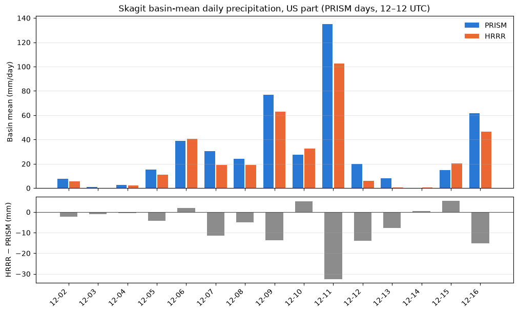
Event totals: PRISM 464 mm, HRRR 370 mm (-20 %)
Interpretation
For this event (US part of the Skagit basin, December 1–16, 2025; precisely 2025-12-01 12:00 to 2025-12-16 12:00 UTC, the part of the request that whole PRISM days cover, since PRISM days run 12–12 UTC), HRRR is about 20 % drier than PRISM (~370 vs. ~464 mm basin mean). That ~94 mm gap is a difference between the two products. Regridding barely affects it: each product’s total from section 1 (native grids) and from this section (aligned grid) differ by only ~2 % (PRISM ~468 vs. ~464 mm, HRRR ~377 vs. ~370 mm). That small change comes from averaging over the exact basin outline on the native grids, but over whole 3 km cells on the aligned grid.
When: about two-thirds of the deficit falls on the three heaviest atmospheric-river days (12-09, 12-11 and 12-16, with the largest gap on 12-11). HRRR is wetter on a few moderate days (12-06, 12-10, 12-15).
Where: the difference map shows HRRR drier mainly in the west and north of the basin, where PRISM is wettest, with scattered patches where HRRR is wetter.
Against the gauges: PRISM is ~9 % above and HRRR ~11 % below the station totals. Across stations PRISM correlates better (0.86 vs. 0.76), but one gauge dominates that: at THBW1 HRRR is ~195 mm above the gauge, while it is below the gauge almost everywhere else. Without THBW1 the correlations are equal (0.89 vs. 0.88) and HRRR is ~15 % low. There are 19 gauges, but three pairs share a location (DARW1/COOPDARW1, MARW1/COOPMARW1, UBKW1/UBDW1), so only 16 sites. Neither product can be called right; the basin truth plausibly lies between the two.
PRISM has no data in British Columbia (~13 % of the basin), so every comparison here covers the US part only.